GraphicsComplex

WLJS

Execution environment

wljs-graphics3d-threejs

Package

Supports dynamics

GraphicsComplex[data_List, primitives_, opts___]

represents an efficient graphics structure for drawing complex 3D objects (or 2D - see GraphicsComplex) storing vertices data in data variable. It replaces indexes found in primitives (can be nested) with a corresponding vertices and colors (if specified)

Most plotting functions such as ListPlot3D and others use this way showing 3D graphics.

The implementation of GraphicsComplex is based on a low-level THREE.js buffer position attribute directly written to a GPU memory.

Supported primitives

Line

No restrictions

v = PolyhedronData["Dodecahedron", "Vertices"] // N;
i = PolyhedronData["Dodecahedron", "FaceIndices"];

GraphicsComplex[v, {Black, Line[i]}] // Graphics3D 

Polygon

Triangles works faster than quads or pentagons

GraphicsComplex[v, Polygon[i]] // Graphics3D 

Non-indexed geometry

One can provide only the ranges for the triangles to be rendered

GraphicsComplex[v, Polygon[1, Length[v]]] // Graphics3D 

warning

it assumes you are using triangles

Point

Sphere

Tube

Options

"VertexColors"

Defines sets of colors used for shading vertices

info

"VertexColors" is a plain list which must have the following form

"VertexColors" ->{{r1,g1,b1}, {r2,g2,b2}, ...}

Supports updates

"VertexNormals"

Defines sets of normals used for shading

Supports updates

"VertexFence"

Defaults to False. When enabled, it sets an update barrier for all dependent primitives, ensuring they update their data only after the vertex data has been updated.

tip

This helps prevent desynchronization issues where the vertex buffer updates lag behind polygon or line indices (or vice versa), which can lead to visual artifacts and WebGL buffer errors.

Dynamic updates

Basic fixed indexes

It does support updates for vertices data and colors. Use Offload wrapper.

cell 1

(* generate mesh *)
proc = HardcorePointProcess[50, 0.5, 2];
reg = Rectangle[{-10, -10}, {10, 10}];
samples = RandomPointConfiguration[proc, reg]["Points"];

(* triangulate *)
Needs["ComputationalGeometry`"];
triangles2[points_] := Module[{tr, triples},
  tr = DelaunayTriangulation[points];
  triples = Flatten[Function[{v, list},
      Switch[Length[list],
        (* account for nodes with connectivity 2 or less *)
        1, {},
        2, {Flatten[{v, list}]}, 
        _, {v, ##} & @@@ Partition[list, 2, 1, {1, 1}]
      ]
    ] @@@ tr, 1];
  Cases[GatherBy[triples, Sort], a_ /; Length[a] == 3 :> a[[1]]]]

triangles = triangles2[samples];

(* sample function *)
f[p_, {x_,y_,z_}] := z Exp[-(*FB[*)(((*SpB[*)Power[Norm[p - {x,y}](*|*),(*|*)2](*]SpB*))(*,*)/(*,*)(2.))(*]FB*)]

(* initial data *)
probe = {#[[1]], #[[2]], f[#, {10, 0, 0}]} &/@ samples // Chop;
colors = With[{mm = MinMax[probe[[All,3]]]},
      (Blend[{{mm[[1]], Blue}, {mm[[2]], Red}}, #[[3]]] )&/@ probe /. {RGBColor -> List} // Chop];

cell 2

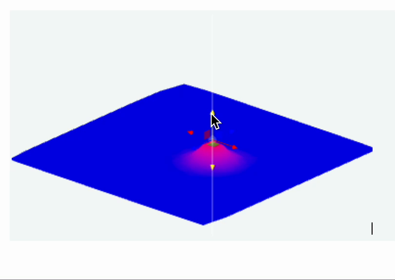
Graphics3D[{
  GraphicsComplex[probe // Offload, {Polygon[triangles]}, "VertexColors"->Offload[colors]],

  EventHandler[Sphere[{0,0,0}, 0.1], {"transform"->Function[data, With[{pos = data["position"]},
    probe = {#[[1]], #[[2]], f[#, pos]} &/@ samples // Chop;
    colors = With[{mm = MinMax[probe[[All,3]]]},
      (Blend[{{mm[[1]], Blue}, {mm[[2]], Red}}, #[[3]]] )&/@ probe /. {RGBColor -> List} // Chop];
  ]]}]
}]

The result is interactive 3D plot

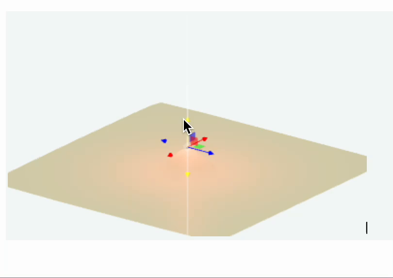
Or the variation of it, if we add a point light source

light = {0,0,0};
Graphics3D[{
  GraphicsComplex[probe // Offload, {Polygon[triangles]}],
  PointLight[Red, light // Offload],

  EventHandler[Sphere[{0,0,0}, 0.1], {"transform"->Function[data, With[{pos = data["position"]},
    probe = {#[[1]], #[[2]], f[#, pos]} &/@ samples // Chop;
    light = pos;
  ]]}]
}]

Update indexes and vertices

For more complicated example you can update both. Here is an example with dynamic adapter for ParametericPlot3D

define shapes

cell 1

sample[t_] := With[{
   complex = ParametricPlot3D[
     (1 - t) * {
       (2 + Cos[v]) * Cos[u],
       (2 + Cos[v]) * Sin[u],
       Sin[v]
     } + t * {
       1.16^v * Cos[v] * (1 + Cos[u]),
       -1.16^v * Sin[v] * (1 + Cos[u]),
       -2 * 1.16^v * (1 + Sin[u]) + 1.0
     },
     {u, 0, 2\[Pi]},
     {v, -\[Pi], \[Pi]},
     MaxRecursion -> 2,
     Mesh -> None
   ][[1, 1]]
   },
  {
   complex[[1]],
   Cases[complex[[2]], _Polygon, 6] // First // First,
   complex[[3, 2]]
  }
]

now construct the scene

LeakyModule[{
    vertices, normals, indices
  },
    {
      EventHandler[InputRange[0,1,0.1,0], Function[value,
        With[{res  = sample[value]},
          normals = res[[3]];
          indices = res[[2]];
          vertices = res[[1]];
        ];
      ]],

      {vertices, indices, normals} = sample[0];
      
      Graphics3D[{
        MeshMaterial[MeshToonMaterial[]], Gray, 
        SpotLight[Red, 5 {1,1,1}], SpotLight[Blue, 5 {-1,-1,1}], 
        SpotLight[Green, 5 {1,-1,1}], 
        PointLight[Magenta, {10,10,10}],
        
        GraphicsComplex[vertices // Offload, {
          Polygon[indices // Offload]
        }, VertexNormals->Offload[normals]]
        
      }, Lighting->None]
    } // Column // Panel 
]

Non-indexed

This is a another mode of working with Non-indexed geometry in Polygon. The benefit of this approach, you can use fixed length buffer for vertices and limit your drawing range using two arguments of Polygon.

tip

Use non-indexed geometry if your polygon count reaches 1 million.

Paint 3D

Marching Cubes examples