Dynamics
The way dynamics work here is quite different from Wolfram Mathematica. Key changes were made for the sake of performance, flexibility—and perhaps a bit of @JerryI’s imagination (one of the maintainers).
However we have some shortcuts to help beginners or Mathematica users to pick up.
If you're looking for the easiest way
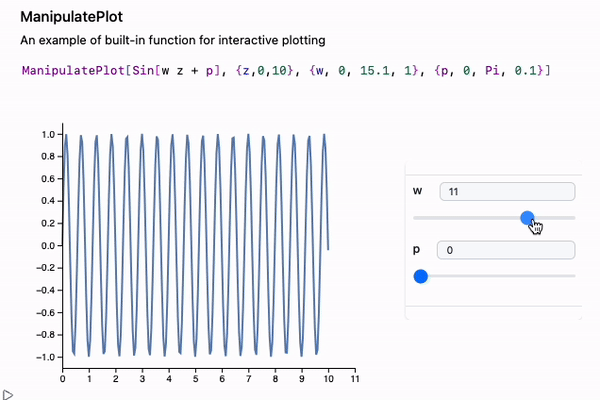
If you want to see how curves change with parameters, check out ManipulatePlot or ManipulateParametricPlot
ManipulatePlot[Sin[w z + p], {z,0,10}, {w, 0, 15.1, 1}, {p, 0, Pi, 0.1}]
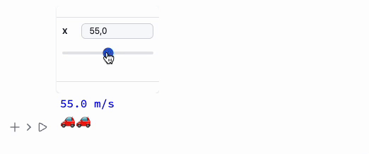
or general-purpose Manipulate, which is great for any valid Wolfram Expression:
Manipulate[Column[{
  Style[StringTemplate["`` m/s"][x], Blue],
  Table["🚗", {i, Floor[x/25]}]//Row
}], {x,10,100}, ContinuousAction->True] // Quiet
It has a built-in Just-in-Time (JIT) transpiler, which optimizes expressions for repeated evaluation using all kinds of tricks with SVG graphics and WebGL:
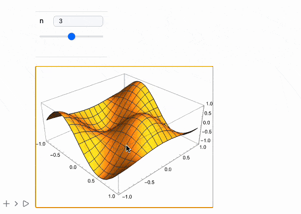
Manipulate[Plot3D[Sin[n x] Cos[n y], {x,-1,1}, {y,-1,1}], {n, 1, 5, 0.3}, ContinuousAction->True]
For small expressions that need to update on a timer or trigger, use Refresh:
Refresh[Now // TextString, 1]
This will update the time in the output cell every second.
... or Animate
If you’re looking to create standalone animations that can be embedded or exported, use AnimatePlot:
AnimatePlot[{Sin[x c], Sinc[x c]}, {x, -10, 10}, {c, 1, 10, 0.1}]
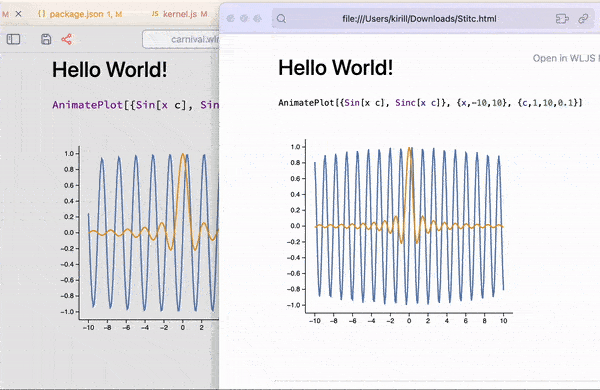
This is all exportable to a compact HTML format 🔥 See how at Interactive HTML
Using Wolfram Language and WLJS you can animate anything - see Animation
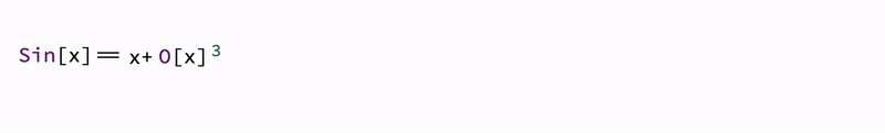
Animate[Row[{Sin[x], "==", Series[Sin[x], {x,0,n}], Invisible[1/2]}], {n, 1, 10, 1}, RefreshRate->3]
Fallback to Mathematica's Rendering
Details
Using MMAView wrapper allows to rasterize interactive output using Wolfram Engine in real-time keeping the original looks of Mathematica's plots
Manipulate[Plot3D[Sin[n x] Cos[n y], {x,-1,1}, {y,-1,1}], {n, 1, 5, 1}] // MMAView
The same works for Animate
Animate[Plot[Sin[x y], {x,0,1}], {y,0,5}] // MMAView
Please do not overuse MMAView since it uses raw raster images streamed in real-time, which is a heavy load to the system. Try to use mostly WLJS's dynamics if possible
Architecture
All dynamics—similar to what you’d expect in Mathematica—are handled mostly on the frontend, i.e., in your browser.
Some expressions are designed to run directly on the frontend, without needing Kernel-side evaluation. In other cases, you can use Offload expression to explicitly tell the Kernel to pass unevaluated expressions to the frontend. This allows flexible structuring of your code to balance performance and control where and how your code is executed.
Learn more here
Keep track of which parts of your code execute on the Wolfram Kernel (server) vs. the frontend (browser). This is crucial for writing predictable and performant code.
In the contrast WLJS Notebook uses more retained mode for handling updates of UI or graphs, rather that immediate mode, which is widely adopted in Mathematica.
Automatic Tracking of Held Symbols
This doesn’t mean Set will automatically reevaluate on nested symbol changes, but many graphics primitives work out of the box. Use Offload to evaluate symbols on the frontend:
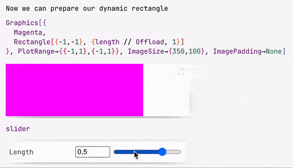
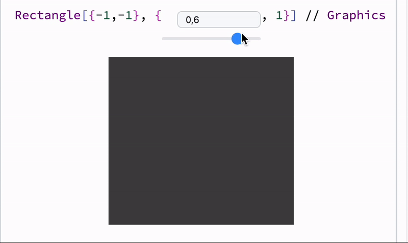
length = 1;

Graphics[{Cyan,
  Rectangle[{-1, -1}, {length // Offload, 1}]
}]
Offload wraps the inner expression and keeps it unevaluated, then it appears to be unknown to the frontend, forcing it to fetch and track it as a dependency.
Now try to evaluate in a new cell
length = 0.5;
Note: The binding here is between Rectangle and length, not the whole Graphics expression. Learn more in the advanced section of the documentation.
Not all primitives or their properties support dynamics. Check the Reference section to confirm:
Please, open an issue on Github page if you need more support of these features
Event-Based Approach
You can use GUI elements (see more at Mouse and keyboard) as event generators:
slider = InputRange[-1, 1, 0.1, "Label" -> "Length"]
EventHandler[slider, Function[l, length = l]];
Once an event is fired, the handler function is executed.
The slider symbol is a special object with both a representation and an event ID.
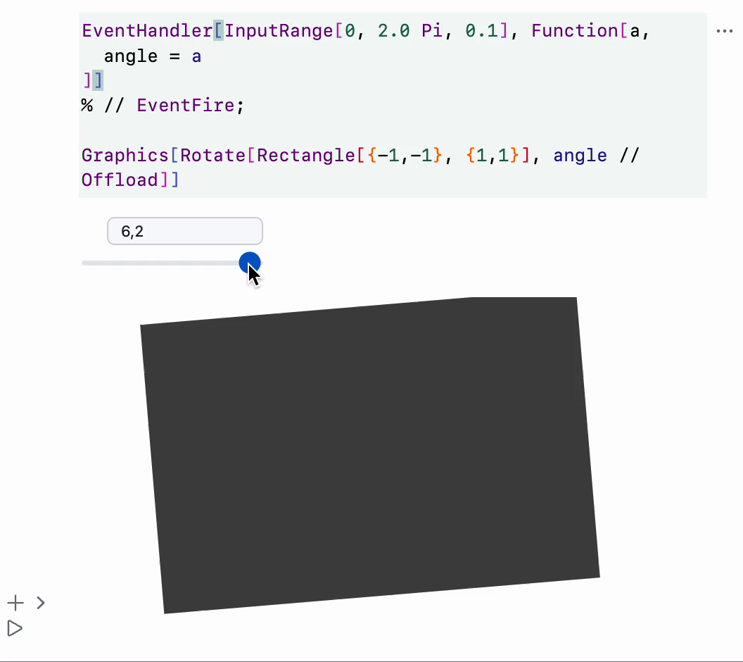
🍪 Example 0 – Simple Rotation
EventHandler[InputRange[0, 2.0 Pi, 0.1], Function[a,
  angle = a
]]
% // EventFire;

Graphics[Rotate[Rectangle[{-1, -1}, {1, 1}], angle // Offload]]
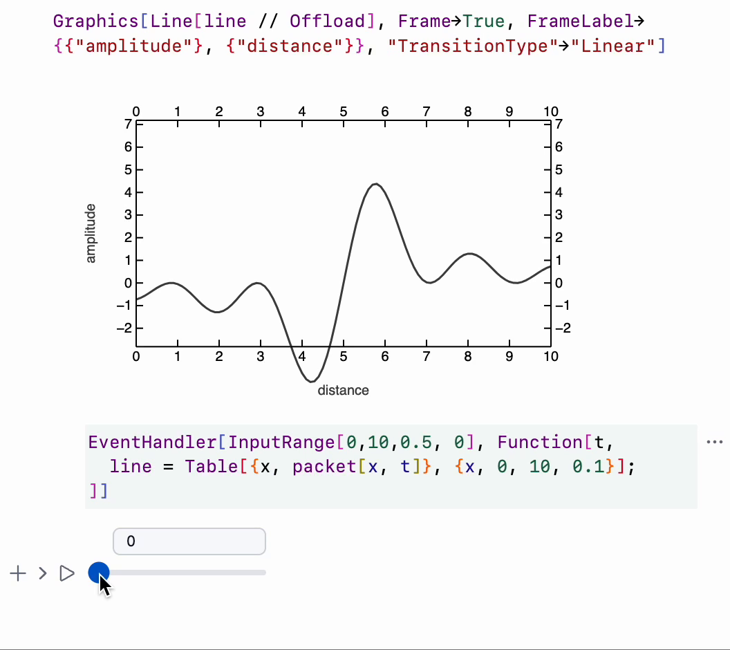
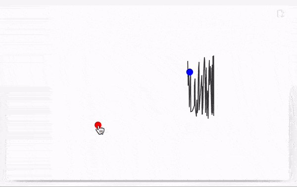
🍪 Example 1 – Wave Packet
packet[x_, t_] := Sum[Sin[-w t + w x], {w, 0, 3, 0.05}] / 10;
line = Table[{x, packet[x, 0]}, {x, 0, 10, 0.1}];

Graphics[Line[line // Offload], Frame -> True, FrameLabel -> {{"amplitude"}, {"distance"}}]
EventHandler[InputRange[0, 5, 0.5, 0], Function[t,
  line = Table[{x, packet[x, t]}, {x, 0, 10, 0.1}];
]]
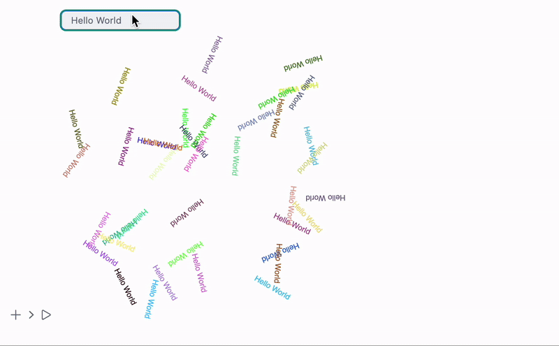
🍪 Example 2 – Hello World Spray
Module[{
  text = "Hello World"
},
  Column[{
    EventHandler[InputText[text], (text = #)&],
    Graphics[Table[{
      RandomColor[],
      Rotate[
        Text[text // Offload, RandomReal[{-1, 1}, 2]],
        RandomReal[{0, 3.14}]
      ]
    }, {40}]]
  }]
]
Event Handlers for Graphics Primitives
p = {0, 0};
Graphics[{
  White,
  EventHandler[
    Rectangle[{-2, -2}, {2, 2}],
    {"mousemove" -> Function[xy, p = xy]}
  ],
  PointSize[0.05], Cyan,
  Point[p // Offload]
}]
Available events:
dragzoomclickmousemovemouseover
For 3D:
transform
Graphics primitive handlers are part of the wljs-graphics-d3 library.
More info in Mouse and Keyboard.
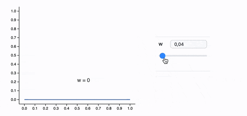
Combination of manual and automated dynamics
Our built-in ManipulatePlot function allows to make basic interactive plots in a single line of code, however, you can add your own dynamic features manually if needed.
For example
Module[{label, pos},
  ManipulatePlot[x w, {x,0,1}, {w,0,2},
    Epilog->Text[Style[label // Offload, FontSize->14], pos // Offload],
    "UpdateFunction" -> Function[input,
      label = StringTemplate["w = ``"][SetPrecision[input,2]];
      pos = {0.5, input 0.5 + 0.2};
      True
    ]
  ]
]
Auto-Generating Dynamic Symbols
Use OffloadFromEventObject to turn event objects into dynamic symbols:
🍪 Example 3 – FABRIK Solver
chain = {Cos[#[[1]]], Sin[#[[2]]]} & /@ RandomReal[{-1, 1}, {65, 2}] // Sort;
lengths = Norm /@ (Reverse[chain] // Differences) // Reverse;
fabrik[lengths_, target_, origin_] := Module[{buffer, prev},
  buffer = Table[With[{p = chain[[-i]]},
    If[i === 1,
      prev = target;
      target
    ,

      prev = prev - Normalize[(prev - p)] lengths[[1-i]];
      prev
    ]
  ], {i, chain // Length}] // Reverse;

  Table[With[{p = buffer[[i]]},
    If[i === 1,
      prev = origin;
      origin
    ,

      prev = prev - Normalize[(prev - p)] lengths[[i-1]];
      prev
    ]
  ], {i, chain // Length}]
]
Graphics[{
  Line[chain // Offload],
  Red, PointSize[0.06],
  EventHandler[Point[{-1, -1}], {"drag" -> Function[xy, chain = fabrik[lengths, xy, First[chain]]]}],
  Blue, Point[origin // Offload]
}, PlotRange -> {{-2, 2}, {-2, 2}}, ImageSize -> 500, "TransitionType" -> "Linear", "TransitionDuration" -> 30]
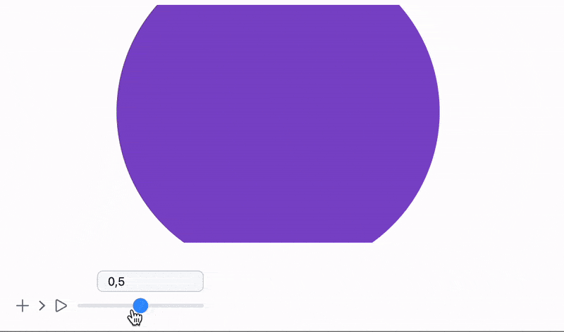
🍪 Example 4 – Opacity Animation
opacity = 0.5;
Graphics[{
  Opacity[Offload[opacity]], Red, Disk[{0, 0}, Offload[1 - opacity]],
  Blue, Opacity[Offload[1.0 - opacity]], Disk[{0, 0}, Offload[opacity]]
}, ImagePadding -> None]

EventHandler[InputRange[0, 1, 0.1], Function[value,
  opacity = value;
]]
All examples are shipped with the app. Locate them here:
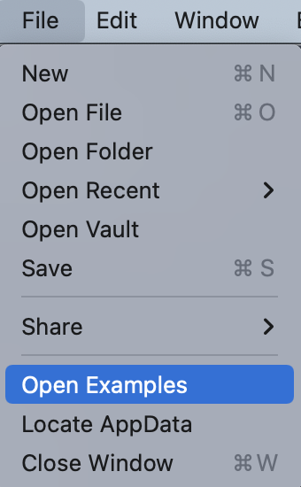
Or access them from the top-bar menu.
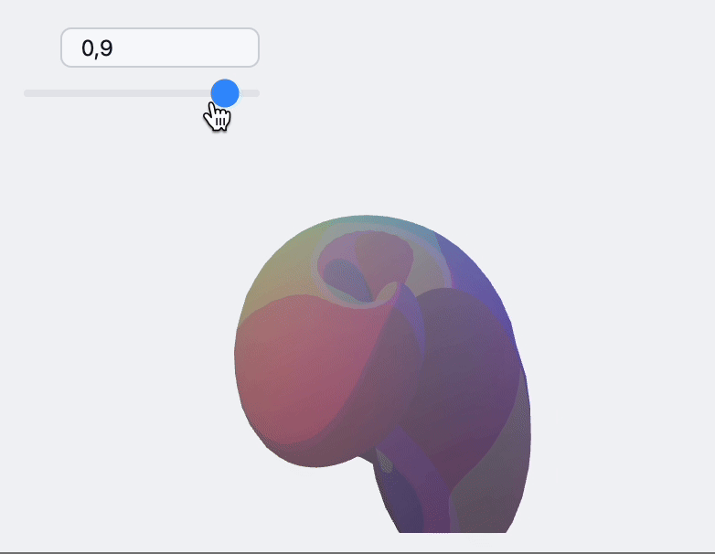
🍪 Example 5 – 3D Morph Mesh
sample[t_] := With[{
   complex = ParametricPlot3D[
     (1 - t) * {
       (2 + Cos[v]) * Cos[u],
       (2 + Cos[v]) * Sin[u],
       Sin[v]
     } + t * {
       1.16^v * Cos[v] * (1 + Cos[u]),
       -1.16^v * Sin[v] * (1 + Cos[u]),
       -2 * 1.16^v * (1 + Sin[u]) + 1.0
     },
     {u, 0, 2\[Pi]},
     {v, -\[Pi], \[Pi]},
     MaxRecursion -> 2,
     Mesh -> None
   ][[1, 1]]
   },
  {
   complex[[1]],
   Cases[complex[[2]], _Polygon, 6] // First // First,
   complex[[3, 2]]
  }
]
Module[{
    vertices, normals, indices
  },
    {
      EventHandler[InputRange[0,1,0.1,0], Function[value,
        With[{res  = sample[value]},
          normals = res[[3]];
          indices = res[[2]];
          vertices = res[[1]];
        ];
      ]],

      {vertices, indices, normals} = sample[0];

      Graphics3D[{
        SpotLight[Red, 5 {1,1,1}], SpotLight[Blue, 5 {-1,-1,1}],
        SpotLight[Green, 5 {1,-1,1}], PointLight[Magenta, {10,10,10}],
        GraphicsComplex[vertices // Offload, {
          Polygon[indices // Offload]
        }, VertexNormals->Offload[normals]]
      }, Lighting->None]
    } // Column // Panel
]
How to Embed on a Web Page?
No Kernel connection needed. Use AnimatePlot or Interactive HTML.
Explore our Blog 📻 for more examples and dev notes.
How to Turn It Into an App?
See Mini Apps