
Here we shall try to model a system of interconnected bonds using the Verlet method. Then, we'll add some visuals to make it feel like a game.
Motion Equations
The system of connected points must obey Newton's laws and kinematic equations as well. To integrate them in real-time, Euler's method, RK (Runge-Kutta), or Verlet methods can be used. We will go for the Verlet method since it will be easier to apply constraints of the bonds in the future:
Download original notebookWe can try to apply it for the simples case, when is sort of a gravity force caused by a red star in the center
estimateX[n_Integer, initialV_:0.01] := FixedPoint[Function[x,
  {
    2 x[[1]] - x[[2]] - 0.001 (*FB[*)((x[[1]])(*,*)/(*,*)((*SpB[*)Power[Norm[x[[1]]](*|*),(*|*)4](*]SpB*)))(*]FB*),
    x[[1]],
    x[[2]]
  }
], {
  {-1.0, 2 initialV 0.01},
  {-1.0, initialV 0.01},
  {-1.0, 0}
}, n];
Now let's plot our solutions for different initial conditions:
Table[{v, Table[estimateX[n, v][[1]], {n, 1, 100}]}, {v,0,4}];
% // Transpose;
ListLinePlot[
  %[[2]]
, PlotStyle -> AbsoluteDashing[{3}]
, PlotRange -> 2{{-1,1}, {-1,1}}
, PlotLegends -> (StringTemplate["v = ``"][#]&/@ %[[1]])
, Epilog -> {Red, Disk[{0,0}, 0.1]}
, Frame -> True
, AspectRatio -> 1
]
(*VB[*)(Legended[ToExpression[FrontEndRef["a289a64a-f3a4-4c9c-8c20-4828fed6ef89"], InputForm], Placed[LineLegend[{Directive[PointSize[1/120], RGBColor[0.24, 0.6, 0.8], AbsoluteThickness[2], AbsoluteDashing[{3}]], Directive[PointSize[1/120], RGBColor[0.95, 0.627, 0.1425], AbsoluteThickness[2], AbsoluteDashing[{3}]], Directive[PointSize[1/120], RGBColor[0.455, 0.7, 0.21], AbsoluteThickness[2], AbsoluteDashing[{3}]], Directive[PointSize[1/120], RGBColor[0.922526, 0.385626, 0.209179], AbsoluteThickness[2], AbsoluteDashing[{3}]], Directive[PointSize[1/120], RGBColor[0.578, 0.51, 0.85], AbsoluteThickness[2], AbsoluteDashing[{3}]]}, {"v = 0", "v = 1", "v = 2", "v = 3", "v = 4"}, LegendMarkers -> {{False, Automatic}, {False, Automatic}, {False, Automatic}, {False, Automatic}, {False, Automatic}}, Joined -> {True, True, True, True, True}, LabelStyle -> {}, LegendLayout -> "Column"], After, Identity]])(*,*)(*"1:eJzVVL9rFEEUvkRNNCgaSWEVo1jYHMa9JewVl+H0LodywXgbrZ3dfZMM2cyEmdmYS2GXP0IbQTuRdEJqCwsLEREUVDD+AgkKNoKd88NbkiOFhYFzio+3771975u3b79TEW+RfYVCQR7RcJ3CzRrEXGDFRTioPU2YA5Z4pN+kDGmoJ1THTCLpM77jGqYEZ6rOkvoKxJnCUQrhGe3GXlDGEz4ukhL2i35cjotB7I0X/cALCCQTQIKyK7xfQyvTrx00BuDkCkvb1jsrMnD8BjTMpDiGhAx0yDQpA8eQHOjUaVKpiDHkIQ01KiBWdBkcW+Oa4ZSpkK6C621bYkU5wyk1SXRFg+tpY40LF3nKhdgYXdu6uvEMiZI9H5G4c9ucr8jVHtZQjSRPMwWz8zReYCAlNT1c/Oi2eA3LecrmXKDDmpqee0Kd2PMdiQc/XkxHxz4hURl6dX+p8rj3qZ80Qx99h/7c4QsSm6sj643Np71P/eWjn5PX1r4h8fbc3Ycn1l8jcbbRd+/Gk/+A+ufnp9/8uvUBiZbd+vedpd/6t9R3/LSheVoeq4yN59b53PJyq5Rb/k7xsArm1GAaiwUQsksU+rc/SRObwqkEO6hqpviinkzc+1n2rkYCL+uPC13Kl4vm3xhdNa2i4gjSULVTIIXdh2dTD+ejbuI2z1Ro+OjVyRaZvUCVKD1/s1KXEmCKqvZvN7mYAw=="*)(*]VB*)
The case of v=3 must be related to the orbital velocity of a star
To see it animated we should repeat the calulations for every frame
With[{initialV = 3.0}, Module[{
  point = {{-1.0, 2 initialV 0.01},
           {-1.0, initialV 0.01},
           {-1.0, 0}}
},
  EventHandler["frameXXX", Function[Null,
    point[[3]] = point[[2]];
    point[[2]] = point[[1]];

    point[[1]] = 2 point[[2]] - point[[3]] - (*FB[*)((point[[1]])(*,*)/(*,*)((*SpB[*)Power[Norm[point[[1]]](*|*),(*|*)4](*]SpB*)))(*]FB*) 0.001;
    point = point; (* to trigger an update *)
  ]];

  Graphics[{
    Point[point // Offload],
    AnimationFrameListener[point // Offload, "Event"->"frameXXX"]
  },
    PlotRange->2{{-1,1}, {-1,1}},
    Epilog -> {Red, Disk[{0,0}, 0.1]},
    AspectRatio->1
  ]
] ]
(*VB[*)(Graphics[{Point[Offload[point$885960]], AnimationFrameListener[Offload[point$885960], "Event" -> "frameXXX"]}, PlotRange -> {{-2, 2}, {-2, 2}}, Epilog -> {RGBColor[1, 0, 0], Disk[{0, 0}, 0.1]}, AspectRatio -> 1])(*,*)(*"1:eJyNUEsOAUEQHX/C2l7iADaElfhbSMjYzLbRPSp6uibdw124icsZXRhiNvTipT6v36uqxgZdkXEcx+QtzFHuBAWmbGGmWbiHrRHZpL8AEz3ZBQsrBPVKSxaWQkhkO1OzcUitZrfb7nVaz+91CwMFAYsA1VSzgJMYV1z/q0ADuEfJ1+Q9OXEVrWlKQVqe532TTIUGlBi5TPk8tcFXBrc4joFKv+sP5SLZhyDRT8nmksO5s+EIJWqgzcBJ4EMfgzmk3N4sfTnTu/ZTtlU6oAn51q5kb/jQvgNiUGVI"*)(*]VB*)
Constraints Algorithm
The simplest and well-known approach for solving the bonds problem is approximating it with springs with finite or infinite stiffness. As it follows from Wikipedia article:
In one dimension, the relationship between the unconstrained positions and the actual positions of points at time step , given a desired constraint distance of , can be found with the algorithm
where is an effective stiffness constant: represents an infinitely stiff spring (hard bond), and represents a soft bond.
Verlet integration is useful because it directly relates the force to the position, rather than solving the problem using velocities.
Constraints Algorithm is applied on the vertices after Verlet integration has been performed
Let's draft a function, that takes the following arguments and process the data efficiently:
- list of vertices
- list of indices of fixed vertices
- list of bonds:
- index A
- index B
- initial length
- stiffness
And it should output a new list of vertices:
processVertices[vertices_List, fixed_List, bonds_List] := Module[{
  coords  = vertices[[1]],
  coords2 = vertices[[2]],
  coords3 = vertices[[3]]
},
  Do[
    coords3 = coords2;
    coords2 = coords;

    Module[{
      integrated = 2 coords2 - coords3 + Table[{0,-1}, Length[coords]] 0.001
    },

      MapThread[Function[{i,j,l,s}, With[{
        d = integrated[[i]] - integrated[[j]]
      },{
        norm = Norm[d]
      },{
        m = 0.5 s Min[(l/(norm+0.001) - 1), 0.1]
             (* avoid blowing up the system *)
      },

        integrated[[i]] +=  m d;
        integrated[[j]] -=  m d;

      ]], RandomSample[bonds]// Transpose];

      Map[Function[index,
        integrated[[index]] = coords[[index]];
      ], fixed];

      coords = integrated;
    ];

  , {2 5}];

  {coords, coords2, coords3}
]
For the stabillity it is recommended to apply constaints in random order
Let us try it on some basic example:
bridge = Join @@ Table[{{i, 75}, {i+5, 55}}, {i,1,100, 10}];
bonds = Join[
  Table[{i, i+1}, {i, 1, Length[bridge]-1, 2}],
  Table[{i, i+2}, {i, 1, Length[bridge]-2, 2}],
  Table[{i+1, i+3}, {i, 1, Length[bridge]-3, 2}]
];
bonds = Map[Join[#, {Norm[bridge[[#[[1]]]] - bridge[[#[[2]]]]], 0.7}//N]&, bonds];

plotBridge[bridge_] := Graphics[{
  MapThread[{bridge[[#1]], bridge[[#2]]}&, bonds // Transpose] // Line,
  Point[bridge],
  ColorData[97][4], MapIndexed[Text[#2[[1]], #1]&, bridge]
}, PlotRange->{{0,100}, {0,100}}, "Controls"->False];

plotBridge[bridge]
(*VB[*)(FrontEndRef["6e84e0a0-3521-4021-a65f-0616f49b418a"])(*,*)(*"1:eJxTTMoPSmNkYGAoZgESHvk5KRCeEJBwK8rPK3HNS3GtSE0uLUlMykkNVgEKm6VamKQaJBroGpsaGeqaGACJRDPTNF0DM0OzNBPLJBNDi0QAdJcU1A=="*)(*]VB*)
Let's run the simulation for a few iterations and plot the final result, while keeping [, ] vertices fixed at the original positions
Module[{bridgeState = {bridge, bridge, bridge}},
  Do[
    bridgeState = processVertices[bridgeState, {1,2,19,20}, bonds];
  , {10}];

  Show[plotBridge[bridge], plotBridge[bridgeState[[1]]]]
]
(*VB[*)(FrontEndRef["1ecdeb3b-30d7-46c4-a925-3ca9ebe9c9fc"])(*,*)(*"1:eJxTTMoPSmNkYGAoZgESHvk5KRCeEJBwK8rPK3HNS3GtSE0uLUlMykkNVgEKG6Ymp6QmGSfpGhukmOuamCWb6CZaGpnqGicnWqYmpVomW6YlAwCTohaW"*)(*]VB*)
Great! At least it did not collapse 🙂 It would be great to see it live. For this we apply the same strategy with Offload technique
Module[{bridgeState, lines, points, frame = CreateUUID[]},

  EventHandler[frame, Function[Null,
    bridgeState = processVertices[bridgeState, {1,2,19,20}, bonds];
    lines = MapThread[{bridgeState[[1,#1]], bridgeState[[1,#2]]}&, bonds // Transpose];
  ]];

  bridgeState = {bridge, bridge, bridge};
  lines = MapThread[{bridgeState[[1,#1]], bridgeState[[1,#2]]}&, bonds // Transpose];
  points = bridge;

  Show[plotBridge[bridge], Graphics[{
    ColorData[97][1], Point[points // Offload],
    Line[lines // Offload],
    AnimationFrameListener[lines // Offload, "Event"->frame]
  }]]
]
(*VB[*)(FrontEndRef["0cbd6656-d9ac-4df1-a450-a9f8e675ae30"])(*,*)(*"1:eJxTTMoPSmNkYGAoZgESHvk5KRCeEJBwK8rPK3HNS3GtSE0uLUlMykkNVgEKGyQnpZiZmZrpplgmJuuapKQZ6iaamBroJlqmWaSamZsmphobAACOdhYF"*)(*]VB*)
Preparing Graphics
The original inspiration was a puzzle video game developed and published by 2D Boy - The World of Goo. It was first released in 2008. In the game, players must use balls of goo to build structures, such as bridges, towers and etc.
We start from the background, and add some blur to it:
background = Blur[(*VB[*)(FrontEndRef["c9796ba9-a2bd-4a6f-af72-d74f43cc33d3"])(*,*)(*"1:eJxTTMoPSmNkYGAoZgESHvk5KRCeEJBwK8rPK3HNS3GtSE0uLUlMykkNVgEKJ1uaW5olJVrqJholpeiaJJql6SammRvpppibpJkYJycbG6cYAwCRChY6"*)(*]VB*), 10];
clouds = {(*VB[*)(FrontEndRef["21c78e25-7714-4a84-b2d9-8ec1a3f0ef8f"])(*,*)(*"1:eJxTTMoPSmNkYGAoZgESHvk5KRCeEJBwK8rPK3HNS3GtSE0uLUlMykkNVgEKGxkmm1ukGpnqmpsbmuiaJFqY6CYZpVjqWqQmGyYapxmkplmkAQB5+BWt"*)(*]VB*),(*VB[*)(FrontEndRef["25f1a881-7f63-4205-a4b8-bdf510809289"])(*,*)(*"1:eJxTTMoPSmNkYGAoZgESHvk5KRCeEJBwK8rPK3HNS3GtSE0uLUlMykkNVgEKG5mmGSZaWBjqmqeZGeuaGBmY6iaaJFnoJqWkmRoaWBhYGllYAgB4xBTp"*)(*]VB*)};
Rendering
Rendering the scene using retained mode with pure raster graphics is more efficient, especially when applying special effects.
For this reason we use Javascript Canvas API, which is mapped 1:1 to Canvas2D library
Needs["Canvas2D`"->"ctx`"] // Quiet;
Let's define a helper function for rendering bonds:
drawBonds[context_, vert_, edges_, fixed_, {width_, height_}] := (
  ctx`BeginPath[context];
  ctx`SetLineWidth[context, 4];
  ctx`SetStrokeStyle[context, "#2C6C75"];

  Do[
    ctx`MoveTo[context, {0, height} - {-1, 1} vert[[p[[1]]]]];
    ctx`LineTo[context, {0, height} - {-1, 1} vert[[p[[2]]]]];
  , {p, edges}];

  ctx`Stroke[context];

  ctx`SetFillStyle[context, "#1C4E28"];

  (
    ctx`BeginPath[context];
    ctx`Arc[context, {0, height} - {-1, 1} #, 6, 0, 2.0 Pi];
    ctx`Fill[context];
  ) &/@ vert;

  ctx`SetFillStyle[context, RGBColor[0.9, 0.4, 0.4]//Darker];

  (
    ctx`BeginPath[context];
    ctx`Arc[context, {0, height} - {-1, 1} vert[[#]], 4, 0, 2.0 Pi];
    ctx`Fill[context];
  ) &/@ fixed;
);
Here we use the same bridge section and render it using our new raster renderer:
Module[{
  ctx = ctx`Canvas2D[]
},
  drawBonds[ctx, 5 bridge, bonds, {1,2,19,20}, {500,500}];
  ctx`Dispatch[ctx];
  Image[ctx, ImageResolution->{500,500}]
]
(*VB[*)(FrontEndRef["f17c87d7-06cf-41d1-838b-c7c9f553800a"])(*,*)(*"1:eJxTTMoPSmNkYGAoZgESHvk5KRCeEJBwK8rPK3HNS3GtSE0uLUlMykkNVgEKpxmaJ1uYp5jrGpglp+maGKYY6loYWyTpJpsnW6aZmhpbGBgkAgCEmBV+"*)(*]VB*)
As a basic visual effect, we can add a trailing effect to the cursor, similar to how it was done in the original game (to some extent):
drawPointer[context_, trail_, edges_, {width_, height_}] := (
  ctx`BeginPath[context];
  ctx`SetLineWidth[context, 2];
  ctx`SetStrokeStyle[context, RGBColor[0.4, 0.6, 0.9]//Darker];

  Do[
    ctx`MoveTo[context, {0, height} - {-1, 1} t[[1]]];
    ctx`LineTo[context, {0, height} - {-1, 1} t[[2]]];
  , {t, edges}];

  ctx`Stroke[context];
  ctx`SetFillStyle[context, RGBColor[0.4, 0.9, 0.6]//Darker];

  Do[
    ctx`BeginPath[context];
    ctx`Arc[context, {0, height} - {-1, 1} trail[[i]], 6.0/i, 0, 2.0 Pi];
    ctx`Fill[context];
  , {i, Length[trail]}];
);
Module[{
  ctx = ctx`Canvas2D[],
  trail = Table[{0,0}, {10}],
  frame = CreateUUID[],
  target = {0,0},
  state = Table[bridge // N, {3}]
},
  EventHandler[frame, Function[Null,
    ctx`ClearRect[ctx, {0,0}, {500,500}];
    drawBonds[ctx, 5 state[[1]], bonds, {1,2,19,20}, {500,500}];
    drawPointer[ctx, trail, {}, {500,500}];
    ctx`Dispatch[ctx];

    trail = RotateRight[trail, 1];
    trail[[1]] = target;

    state = processVertices[state, {1,2,19,20}, bonds];
  ]];

  EventHandler[Image[ctx,
    ImageResolution->{500,500},
    Epilog->AnimationFrameListener[ctx, "Event"->frame]
  ], {
    "mousemove"->Function[xy,
      target = {0,500} + {1,-1} xy;
  ]}]
]
Utils
For adding more bonds to the structure of a bridge, we need to find the shortest links (maximum 2) to the cursor position. Here is a little function for this purpose:
findConnections[vertx_, p_, th_: 2.0] :=
  With[{a =
     MapIndexed[Function[{val, i},
       With[{n = Norm[p - val]},
        If[n < th, {i[[1]], n}, Nothing]]], vertx]},
   If[Length[a] == 0, {},
    If[Length[a] > 2,
     TakeSmallestBy[a, Function[v, v[[2]]], 2], a][[All, 1]]]]
It is far from the optimal solution, since it naively checks all vertices available.
Wrapping up
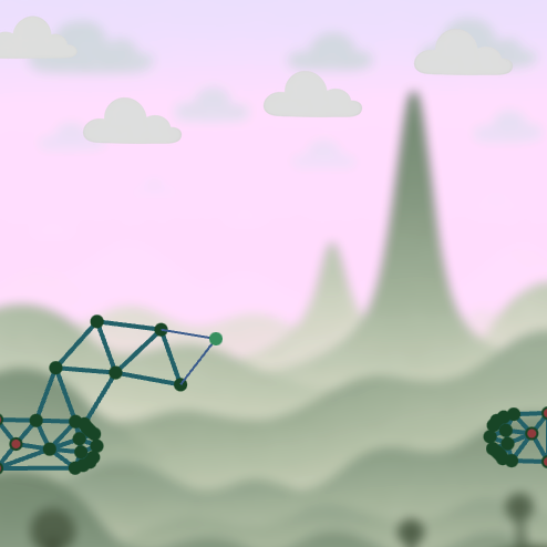
As the last step, we add a click listener to append new vertices and bonds to the system. For the visuals, we also add a background image and moving clouds in a simple linear pattern:
With[{
  frame = CreateUUID[],
  ctx = ctx`Canvas2D[],
  fixed = NotebookStore["contemporaneously-be4"]
}, Module[{
  p, pointer, trail, target, nearbyVertices, bonds,
  offset, targetOffset, cloudsPos, cloudsImages
},
  p = NotebookStore["audience-36d"];
  bonds = NotebookStore["huckster-6b8"];

  nearbyVertices = {};
  cloudsPos = NotebookStore["circumvention-9f5"];

  cloudsImages = RandomChoice[clouds, 5];


  pointer = {250,250};
  offset = 0.0;
  targetOffset = -150;
  target = pointer;
  trail = Table[pointer, {10}];

  EventHandler[frame, Function[Null,

    (* clear and translate the screen buffer *)
    ctx`ClearRect[ctx, {0,0}, {500,500}];
    ctx`Translate[ctx, {0, offset}];

    (* background *)
    ctx`DrawImage[ctx, background, {0,0}];
    MapThread[ctx`DrawImage[ctx, #1, #2]&, {cloudsImages, cloudsPos}];

    (* draw bridge *)
    drawBonds[ctx, p[[1]], bonds, fixed, {500,500}];


    (* draw a cursor *)
    drawPointer[ctx, trail, {trail[[1]], p[[1, #]]} &/@ nearbyVertices, {500,500}];

    (* reset transformation and flip the buffers *)
    ctx`Translate[ctx, {0, -offset}];
    ctx`Dispatch[ctx];

    (* trail computations *)
    pointer = 0.35 (target + {0,1} offset) + 0.65 pointer;
    trail = RotateRight[trail, 1];
    trail[[1]] = pointer;

    (* animation of clouds *)
    cloudsPos = Map[If[#[[1]] > 500, {-150, #[[2]]}, # + {1,0}]&, cloudsPos];

    (* camera animation *)
    If[target[[2]]  < 100 && targetOffset > -200, targetOffset-=6.0];
    If[target[[2]]  > 500-100 && targetOffset < 0, targetOffset+=6.0];

    offset = offset + 0.1 (targetOffset - offset);

    (* perform Verlet *)
    p = processVertices[p, fixed, bonds];
  ]];

  EventHandler[Image[ctx, ImageResolution->{500,500}, Epilog->{
    AnimationFrameListener[ctx, "Event"->frame]
  }], {
    "click" -> Function[xy,
      p[[1]] = Append[p[[1]], pointer];
      p[[2]] = Append[p[[2]], pointer];
      p[[3]] = Append[p[[3]], pointer];
      With[{length = Length[p[[1]]]},
        bonds = Join[bonds, Table[
          {length, i, Norm[pointer - p[[1, i]]], 0.3}
        , {i, nearbyVertices}]];
      ];
    ],
    "mousemove" -> Function[xy,
      target = {0, 500} - {-1, 1} xy;
      (* scan for vertices near the cursor *)
      nearbyVertices = findConnections[p[[1]], pointer, 60];
    ]
  }]
]]
This wasn't that hard, was it? It is amazing how powerful Wolfram Language becomes once bridged with web-tech sandbox tools
If you are reading this from a web page and not from the WLJS Notebook:
Some resources were kept within the notebook storage. Download the original notebook from the heading section to have all images and precalculated vertices.