1 Minute of Verlet Integration: Supplementary materials

· 7 min read

Maintainer

I've made a video recently on one of my favourite methods for solving Newton's equations. It is available on YouTube Shorts 🎥

It wasn't clear to me if this is worth a full article or just a short comment. Let me start with a supplementary material for the video first, and then we shall see...

Actual Video

Download original notebook

I've already published a blog post on the Verlet method, briefly mentioning the ideas behind it.

Basics

All credit goes to these people:

As shown in the video, a simple idea leads us to the following numerical solution of both kinematic and dynamic problems:

x_{n+1} = 2 x_{n} - x_{n-1} + \delta^{2} f_{n}/m

where $n$ represents the number of iterations.

Implementation

The aforementioned equation translates nicely into computer code. Here, for demonstration purposes, I am going to use our beloved sandbox, the WLJS Notebook:

With[{uid = CreateUUID[], ball = Unique["ball"]},
  ball = Table[{0,0}, {3}];
  
  EventHandler[uid, Function[Null,
    ball[[3]] = ball[[2]];
    ball[[2]] = ball[[1]];
    
    ball[[1]] = 2 ball[[2]] - ball[[3]] + {0,-1} 0.01;
    If[ball[[1, 2]] < -1.0, ball[[{1,2}]] = ball[[{2,1}]]]; 
    
    ball = ball;
  ]];

  Graphics[{
    {Gray, Line[{{-1,0}, {1,0}}]},
    Point[ball[[1]]//Offload],
    AnimationFrameListener[ball//Offload, "Event"->uid]
  }, PlotRange->{{-1,1}, {-1,1}}]
]

(*VB[*)(Graphics[{{GrayLevel[0.5], Line[{{-1, 0}, {1, 0}}]}, Point[Offload[ball57[[1]]]], AnimationFrameListener[Offload[ball57], "Event" -> "55d577c9-f698-407b-b32f-b86a5f472c4a"]}, PlotRange -> {{-1, 1}, {-1, 1}}])(*,*)(*"1:eJyNkEtuwjAQhkNLH1yAfaVuIyEaY1ghFtAuIhGFE4wTGywZGzluJG7LTcB2gJBkwyx+zcP/N9Z8EZWyXhAERd/KnxI5e3HVp5VfDYcdzwr2epvHvDDV/F5576B6fYxpSYUOfJzmNTfmkrZ8jYqfbXDnavUdoep71puVRHF5XfthZc2YUJDXvgS0Kd5tQkAIhD2img6tLCTfg+FKrjTsqdtBJdUd3AOgJqf/gm7cF5YllWbzbTOEcoRxNgvZZDYNoxEmIfkZs5BMJ4BYhMdZBE2Av1UilElBbp84Sq97lHv/AnqhZB4="*)(*]VB*)

All positions of a single bouncing ball are stored in the ball symbol. The resulting equations for this case are as follows:

\begin{align*} &ball_{n-1} &=& ~ ball_{n} \\ &ball_{n} &=& ~ball_{n+1} \\ &ball_{n+1} &=& ~2 ball_{n} - ball_{n-1} + \begin{bmatrix}0 \\ -1 \end{bmatrix} \alpha^2 \end{align*}

where the last term $\alpha$ represents the gravitational force.

Additionally, we consider the boundary conditions: if a ball crosses the ground, we exchange $ball_{n}$ and $ball_{n+1}$ , which implicitly flips the velocity

Loses

To consider inelastic case we should simply reduce the reflected momentum (or velocity in our case).

General Boundary Conditions

I guess for the simplest case, our trick with flipping the velocity works well. However, for a surface at an angle, it might not work well, since we need to mirror the velocity along the plane defined by some kind of normal vector.

It is a nice exercise you can try at home:

But here I will just give an answer:

\mathbf{v}^{\prime} = \mathbf{v} - 2~\mathbf{n} (\mathbf{n} \cdot \mathbf{v})

Ball in a rim

A good example to try it could be:

Circle[]//Graphics

(*VB[*)(Graphics[Circle[{0, 0}], ImageSize -> 200])(*,*)(*"1:eJxTTMoPSmNkYGAoZgESHvk5KWlMIB4HkHAvSizIyEwuhsizAQnnzKLknFSICpB6n8zikkwgzQAmEOJBpTmpxZxAhmduYnpqcGZVauYJIA8AhSoV3w=="*)(*]VB*)

Let's try it:

With[{
  p = Unique["bbb"], 
  frame = CreateUUID[],
  circ = {0,0}
},
  p = Table[{0,0}, {3}];

  EventHandler[frame, Function[Null,
    Module[{b = p, \[Delta]t = 0.01},
      Do[
        If[Norm[b[[1]]-circ] > 1.0,
          With[{n = -Normalize[b[[1]]-circ], delta = b[[1]]-b[[2]]},
            b[[2]] = b[[1]];
            b[[1]] = b[[1]] -  n (n.delta);
          ]
        ];

        b[[3]] = b[[2]];
        b[[2]] = b[[1]];
        b[[1]] = 2 b[[2]] - b[[3]] + {0,-1} (*SpB[*)Power[\[Delta]t(*|*),(*|*)2](*]SpB*);
      , {5}];
    
      p = b;
    ];
  ]];

  Graphics[{
    Circle[circ, 1.0], 
    Lighter[Lighter[Red]], Disk[p[[3]]//Offload, 0.01],
    Lighter[Red], Disk[p[[2]]//Offload, 0.01],
    Red, Disk[p[[1]]//Offload, 0.01],
    AnimationFrameListener[p//Offload, "Event"->frame]
  }, PlotRange->{{-1,1}, {-1,1}}, AspectRatio->1]
]

Hm... it is hard to tell if it works. Unless we make our boundary circle movable:

With[{
  p = Unique["bbb"], 
  frame = CreateUUID[],
  circ = Unique["bbb"]
},
  circ = {0,0};
  p = Table[{0,0}, {3}];

  EventHandler[frame, Function[Null,
    Module[{b = p, \[Delta]t = 0.01},
      Do[
        If[Norm[b[[1]]-circ] > 1.0,
          With[{n = -Normalize[b[[1]]-circ], delta = b[[1]]-b[[2]]},
            b[[2]] = b[[1]];
            b[[1]] = b[[1]] -  n (n.delta);
          ]
        ];

        b[[3]] = b[[2]];
        b[[2]] = b[[1]];
        b[[1]] = 2 b[[2]] - b[[3]] + {0,-1} (*SpB[*)Power[\[Delta]t(*|*),(*|*)2](*]SpB*);
      , {5}];
    
      p = b;
    ];
  ]];

 {
  Graphics[{
    Circle[circ//Offload, 1.0], 
    Lighter[Lighter[Red]], Disk[p[[3]]//Offload, 0.01],
    Lighter[Red], Disk[p[[2]]//Offload, 0.01],
    Red, Disk[p[[1]]//Offload, 0.01],
    AnimationFrameListener[p//Offload, "Event"->frame]
  }, PlotRange->{{-1,1}, {-1,1}}, AspectRatio->1],

  EventHandler[InputJoystick[], Function[xy, circ = xy]]
 } // Column
]

Accuracy of numerics

Even if we slow down time (by decreasing the time steps of the simulation), we might still face issues if, for some reason, $x_{n}$ and $x_{n+1}$ turn out to be both outside the boundaries. It could be the result of some large impact:

note

Yes, we have to cheat as most developers do in physics engines

In the worst case have would have to clamp positions to the boundary regions:

If one knows some better approach, please, let me know in the comments 🧙🏼‍♂️

Momentum Transfer

A rim itself (or a circle, if you wish) also has velocity and momentum. However, for now, it cannot be transferred to our ball.

How can we do that without violating the physics?

Whenever you have troubles, move to some other Frame of Reference

By moving our calculations to the frame of reference of our rim (moving frame), we remove this puzzle completely. Since the velocity of the rim is zero there, it is static object. Then we solve our boundary problem in that frame of reference, and afterward move back to the original static frame of reference:

With[{
  p = Unique["bbb"],
  circ = Unique["bbb"],
  target = Unique["bbb"],
  frame = CreateUUID[]
},
  p = Table[RandomReal[{-1,1}, 2]0.001, {3}, {100}];
  circ = {{0,0}, {0,0}};
  target = {0,0};
  
  EventHandler[frame, Function[Null,
    Module[{b = p, \[Delta]t = 0.005},
      Do[
        circ[[1]] = circ[[1]] + \[Delta]t (target - circ[[1]]);
        
        b[[{1,2}]] = MapThread[If[Norm[#1-circ[[2]]] > 1.0, Module[{
          u = {#1, #2},
          vel = (circ[[1]] - circ[[2]])
        },
  
          (* change frame of reference *)
          u[[1]] = u[[1]] - vel;
          
          
          With[{n = -Normalize[u[[1]]-circ[[2]]], delta = u[[1]]-u[[2]]},
            u[[2]] = u[[1]];
            u[[1]] = u[[1]] -  0.8 n (n.delta);
          ];
  
          (* go back to the original *)
          u[[1]] = u[[1]] + vel;
  
          (* clamp to the boundary region *)
          If[Norm[u[[1]]-circ[[2]]] > 1.0, 
            u[[1]] += (1.0 - Norm[u[[1]]-circ[[2]]]) Normalize[u[[1]]-circ[[2]]];
          ];
  
          u
        ], {#1, #2}]&, {b[[1]], b[[2]]}] // Transpose;
  
        b[[3]] = b[[2]];
        b[[2]] = b[[1]];
        b[[1]] = 2 b[[2]] - b[[3]] + Table[{0,-1}, {Length[b[[1]]]}] (*SpB[*)Power[\[Delta]t(*|*),(*|*)2](*]SpB*);
  
  
        circ[[2]] = circ[[1]];
      , {10}];
  
      circ = circ;
  
      p = b;
    ];
  ]];

  {
    Graphics[{
      Circle[circ[[1]] // Offload, 1.0], 
      Pink, Point[p[[1]] // Offload],
      AnimationFrameListener[p//Offload, "Event"->frame]
    }, PlotRange->{1.4{-1,1}, 1.4{-1,1}}, AspectRatio->1, ImageSize->Medium, TransitionType->None],
  
    EventHandler[InputJoystick[], Function[xy, target = xy;]]
  } // Row
]

Constraint Algorithm

Whenever you try to model a system with multiple hard or soft bonds connecting different nodes, it quickly becomes a pain. This is one of those cases where solving the problem using only positions—without momentum and forces-becomes a game changer.

As mentioned in my previous post:

By directly adjusting the positions of two points connected by a bond to maintain the bond length, we effectively account for all forces in a single step.
The stiffness of the bond is not directly part of the differential equation—it's introduced through how you enforce the constraint: either strictly (hard) or partially (soft).

Firstly, we perform a normal Verlet update and then apply constraints. Since each bond affects both vertices, the "information" (momentum, tension, etc.) travels through all nodes of the system. This allows, for instance, if our mesh hits the ground with one of its vertices, the whole body will stop and bounce back.

In addition, I will give an example similar to what you have seen in the video:

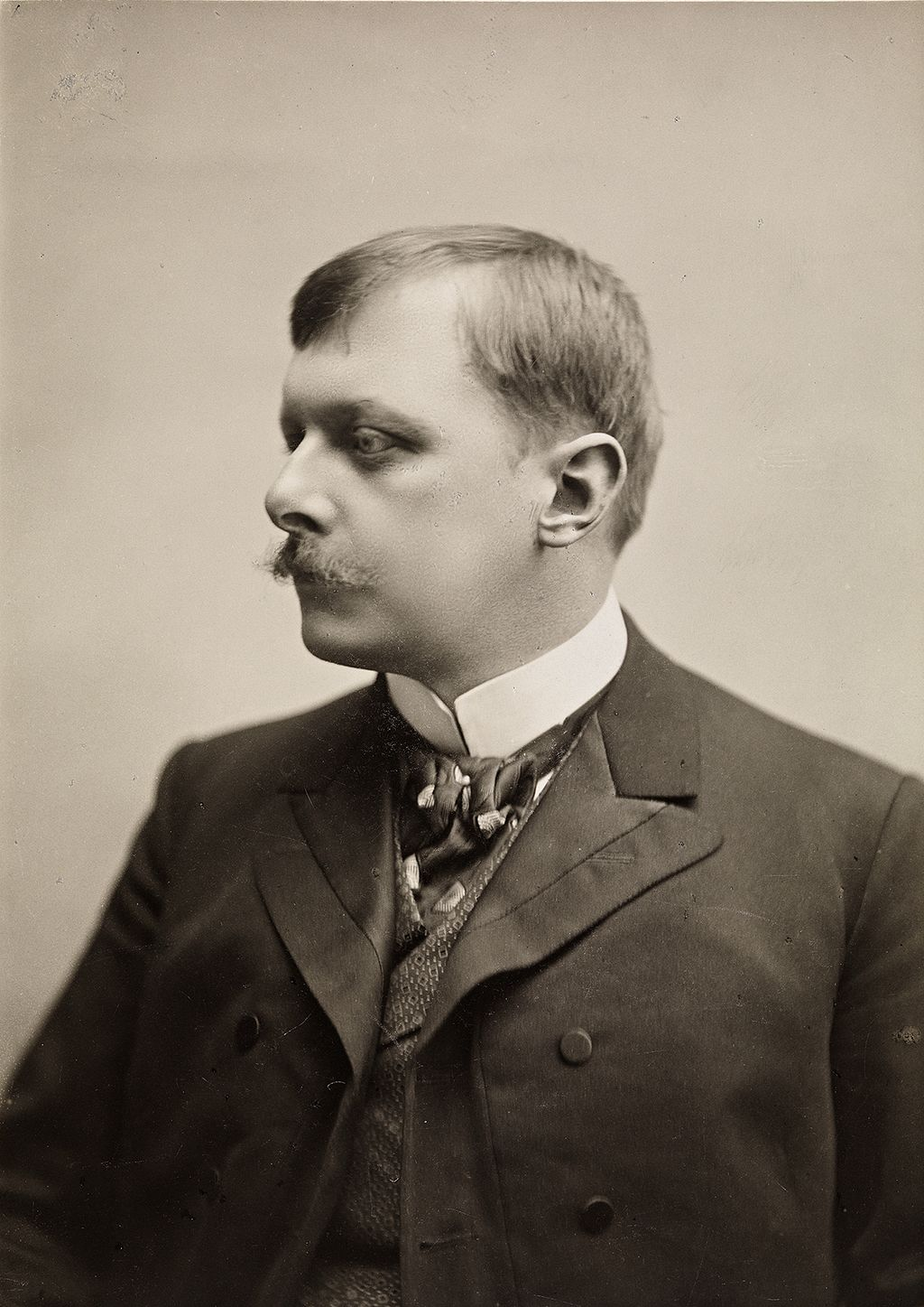
Image to Mesh

Transformation of the b/w image to a mesh of interconnected vertices

tip

Go to the header section to download this notebook

(dude = NotebookStore["cob-105"])//Colorize

(*VB[*)(FrontEndRef["f689ba6c-806f-4606-8ca2-ebf725f42548"])(*,*)(*"1:eJxTTMoPSmNkYGAoZgESHvk5KRCeEJBwK8rPK3HNS3GtSE0uLUlMykkNVgEKp5lZWCYlmiXrWhiYpemamBmY6VokJxrppialmRuZppkYmZpYAACGoRWG"*)(*]VB*)

Now transform it into bonds:

SetAttributes[UndirectedEdge, Orderless];

getMesh[img_] := With[{mesh = TriangulateMesh[ImageMesh[img], MaxCellMeasure->{"Area"->45}]}, Module[{
  vertices = MeshCoordinates[mesh],
  edges = (Cases[mesh//MeshCells, _Polygon, 2] /. {
  Polygon[{a_, b_, c_}] :> Sequence[UndirectedEdge[a,b], UndirectedEdge[b,c], UndirectedEdge[a,c]]
} // DeleteDuplicates) /. {UndirectedEdge -> List}
},
  {vertices, edges}
] ]

And apply to our dude

NotebookStore["dudeMesh"] = dude // getMesh;
dude // getMesh;
Graphics[GraphicsComplex[%[[1]], {Line /@ %[[2]]}]]

(*VB[*)(FrontEndRef["3bb3903f-7fe8-4344-8870-49d66474905c"])(*,*)(*"1:eJxTTMoPSmNkYGAoZgESHvk5KRCeEJBwK8rPK3HNS3GtSE0uLUlMykkNVgEKGyclGVsaGKfpmqelWuiaGJuY6FpYmBvomlimmJmZmJtYGpgmAwB6kxTM"*)(*]VB*)

Rendering

There is an issue with the traditional approach to animating using Graphics when dealing with numerous line segments. Typically, you might use GraphicsComplex, but as of now, it does not support updates. This may change in the future. This means that if the data changes, it won't be reflected. Working with individual Line primitives seems like a good plan (as was done in the previous post), but for the sake of performance, we shall use a 2D raster canvas here:

Needs["Canvas2D`"->"ctx`"] // Quiet;

And here is a little helper function for drawing all bonds:

drawBonds[context_, vert_, edges_] := Module[{},

  ctx`ClearRect[context, {0,0}, {500,500}];

  ctx`BeginPath[context];
  ctx`SetLineWidth[context, 4];
  ctx`SetStrokeStyle[context, (*VB[*)(RGBColor[0.4, 0.6, 0.9])(*,*)(*"1:eJxTTMoPSmNiYGAo5gUSYZmp5S6pyflFiSX5RcEsQBHn4PCQNGaQPAeQCHJ3cs7PyS8qmjUTBG7aFxmDwWP7orNnQOCNPQBuvhsO"*)(*]VB*)];

  Do[
    ctx`MoveTo[context, {0, 500} - {-5, 5} vert[[p[[1]]]]];
    ctx`LineTo[context, {0, 500} - {-5, 5} vert[[p[[2]]]]];
  , {p, edges}];

  ctx`Stroke[context];

  ctx`SetFillStyle[context, (*VB[*)(RGBColor[0.4, 0.9, 0.6])(*,*)(*"1:eJxTTMoPSmNiYGAo5gUSYZmp5S6pyflFiSX5RcEsQBHn4PCQNGaQPAeQCHJ3cs7PyS8qmjUTBG7aF509AwJv7IuMweCxPQCPXhsO"*)(*]VB*)];

  (
    ctx`BeginPath[context];
    ctx`Arc[context, {0, 500} - {-5, 5} #, 6, 0, 2.0 Pi];
    ctx`Fill[context];
  ) &/@ vert;

  ctx`Dispatch[context];
];

Simulation

And now finally the simulation!

generatorSimulation[finalVerts_, finalBonds_] := Module[{
  coords, coords3, coords2
},

coords = finalVerts;
coords2 = finalVerts;
coords3 = finalVerts;

Function[Null, Do[
    coords3 = coords2;
    coords2 = coords;
    
    Module[{new = 2 coords2 - coords3 + Table[{0,-1}, Length[coords]] 0.0001},
      MapThread[Function[{i,j,l}, With[{d = new[[i]]-new[[j]]}, With[{m = Min[((*FB[*)((l)(*,*)/(*,*)(Norm[d]+0.001))(*]FB*) - 1), 0.1]},
        new[[i]] +=  (*FB[*)((1)(*,*)/(*,*)(2))(*]FB*) m d;
        new[[j]] -=  (*FB[*)((1)(*,*)/(*,*)(2))(*]FB*) m d;
      ] ]], RandomSample[finalBonds]// Transpose]; 
      
      new = Map[Function[xy,
        If[xy[[2]] < 0.0, {xy[[1]], 0.0}, xy]
      ], new];
      
      coords = new;
    ];

    , {2 5}];

    coords
]]

Run it in a loop:

{finalVerts, finalPairs} = NotebookStore["dudeMesh"];
finalBonds = {finalPairs[[All,1]], finalPairs[[All,2]], Norm[finalVerts[[#[[1]]]] - finalVerts[[#[[2]]]]]&/@finalPairs} // Transpose;

With[{
  context2D = ctx`Canvas2D[],
  uid = CreateUUID[],
  calc = generatorSimulation[{#[[1]], #[[2]] + 50.0} &/@ finalVerts, finalBonds]
},
  EventHandler[uid, Function[Null,
    drawBonds[context2D, calc[], finalPairs]
  ]];
  Image[context2D, ImageResolution->{500,500}, Epilog->{
    AnimationFrameListener[context2D, "Event"->uid]
  }]
]

Many-body Problem

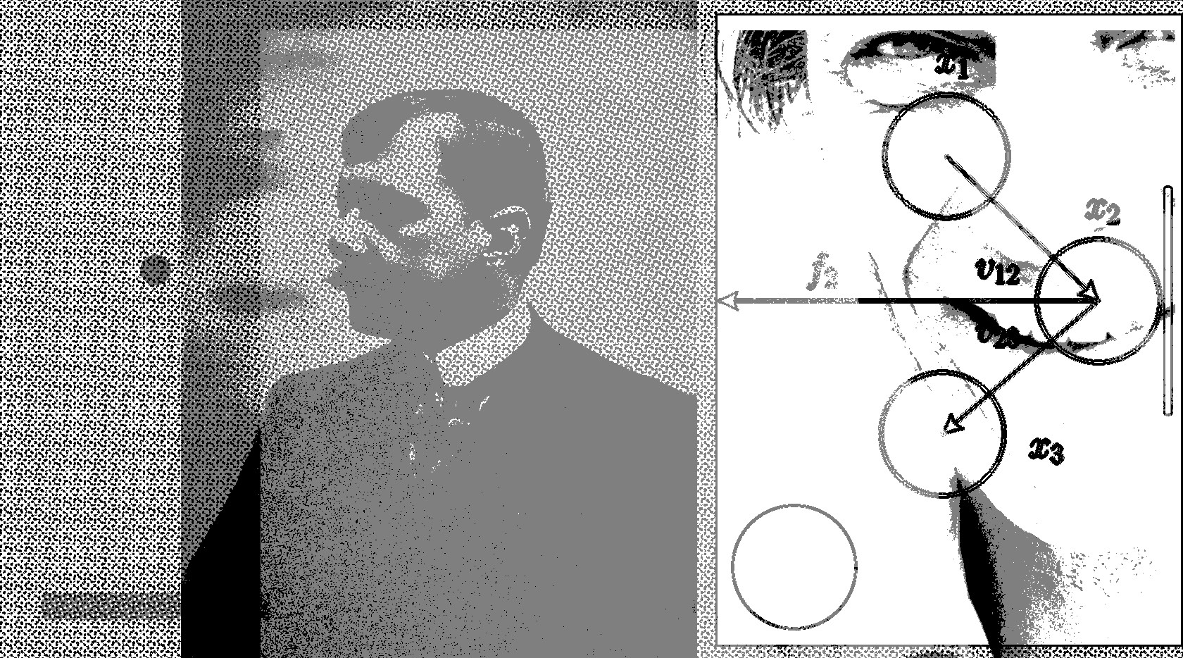
A well-known and common problem in computational physics, and not only there, is dealing with many entities coupled by a two-particle function.

Similarly to the constraints algorithm, one can resolve the collisions between balls or disks by offsetting their positions. This is not a completely physical approach, but it could approximate the case when particles collide in an inelastic way, losing momentum and energy to heat:

Unfortunately, this also means that the complexity of our algorithm scales as $N^2$ , where $N$ is the number of our particles, leading to performance issues. There are many ways to deal with this, but the easiest one would be to compile our little program.

Fortunately, there is a built-in expression Compile that allows us to directly translate Wolfram Language code to C or internal bytecode. Of course, it comes with restrictions on statically typed data structures and other limitations:

compiled = Compile[{
  {p, _Real, 3}, {c, _Real, 2}, {target, _Real, 1}
}, Module[{b = p, \[Delta]t = 0.005, circ = c},
    Do[
      circ[[1]] = circ[[1]] + \[Delta]t (target - circ[[1]]);
      
      b[[{1,2}]] = MapThread[If[Norm[#1-circ[[2]]] > 1.0, Module[{
        u = {#1, #2},
        vel = (circ[[1]] - circ[[2]])
      },

        
        u[[1]] = u[[1]] - vel;
        
        
        With[{n = -Normalize[u[[1]]-circ[[2]]], delta = u[[1]]-u[[2]]},
          u[[2]] = u[[1]];
          u[[1]] = u[[1]] -  0.9 n (n.delta);
        ];

        u[[1]] = u[[1]] + vel;

        If[Norm[u[[1]]-circ[[2]]] > 1.0, (*clamp to the region *)
          u[[1]] += (1.0 - Norm[u[[1]]-circ[[2]]]) Normalize[u[[1]]-circ[[2]]];
        ];

        u
      ], {#1, #2}]&, {b[[1]], b[[2]]}] // Transpose;

      b[[3]] = b[[2]];
      b[[2]] = b[[1]];
      b[[1]] = 2 b[[2]] - b[[3]] + Table[{0,-1}, {Length[b[[1]]]}] (*SpB[*)Power[\[Delta]t(*|*),(*|*)2](*]SpB*);


    (* Particle-particle collisions *)
    Do[
      Do[
        If[i < j,
          Module[{pi = b[[1, i]], pj = b[[1, j]], d, dist, n, overlap},
            d = pj - pi;
            dist = Norm[d];
            If[dist < 0.05,
              n = Normalize[d];
              overlap = 0.05 - dist;
              b[[1, i]] -= 0.5 overlap n;
              b[[1, j]] += 0.5 overlap n;
            ];
          ]
        ],
        {j, Length[b[[1]]]}
      ],
      {i, Length[b[[1]]]}
    ];   


      circ[[2]] = circ[[1]];
    , {10}];

    b[[-1, 1]] = circ[[1]];
    b[[-1, 2]] = circ[[2]];

    b
  ], CompilationOptions -> {"InlineExternalDefinitions" -> True}, 
    "CompilationTarget" -> "C","RuntimeOptions" -> "Speed"];

Please, don't be confised by the design of the input and output of this compiled function. In Wolfram Language Compileed expressions cannot return nested structures, therfore we have to trick and sort of serialize the data into a numerical tensor and then deserialize back. In this case it is done using Part.

The rest is on us, i.e. to plug our function back into the main loop:

With[{
  p = Unique["ppp"],
  toDraw = Unique["ppp"],
  circ = Unique["ppp"],
  target = Unique["ppp"],
  frame = CreateUUID[]
},
  p = Table[Exp[-i/80.0]{Sin[i], Cos[i]}, {3}, {i, 100}];
  toDraw = p[[1]];
  circ = {{0,0}, {0,0}};
  target = {0,0};

  EventHandler[frame, Function[Null,
      With[{
        c = compiled[Join[p, {p[[3]]}], circ, target]
      },
        circ = c[[4, {1,2}]];
        p = c[[1;;3]];
        toDraw = p[[1]];
      ]
  ]];

  {
    Graphics[{
      PointSize[0.03],
      Circle[circ[[1]] // Offload, 1.0], 
      Pink, Point[toDraw // Offload],
      AnimationFrameListener[p//Offload, "Event"->frame]
    }, 
      PlotRange->{1.4{-1,1}, 1.4{-1,1}}, 
      AspectRatio->1, ImageSize->Medium, 
      TransitionType->None
    ],

    EventHandler[InputJoystick[], Function[xy, target = xy;]]
  } // Row
]

As you can see, one can go quite far using this toolbox.
Hope you’ve learned something fun today! 🫶

Feel free to share thoughts or ask questions in the comments.

A Note on the Animation

What you saw in the video (YouTube Short) was created entirely using the WLJS Notebook and its built-in Animation Framework utilities.

If anyone’s interested, I’d be happy to share the source code with the community.

Basics​

Implementation​

Loses​

General Boundary Conditions​

Ball in a rim​

Accuracy of numerics​

Momentum Transfer​

Constraint Algorithm​

Image to Mesh​

Rendering​

Simulation​

Many-body Problem​

A Note on the Animation​