PID Controllers are Fun!
This is one of the most widely used feedback control mechanisms. You will eventually find it everywhere, when you press the gas handle on an e-scooter, set the heater in your room, or even flush a toilet.
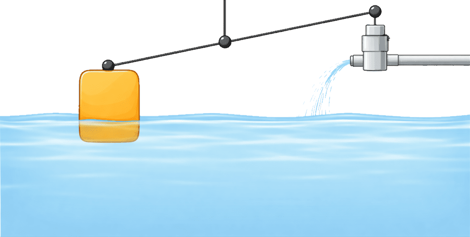
Let's start with a familiar example as on the preview picture. In this example, the water level must be full, i.e., if we have a non-zero error , this will open a valve, i.e., send a control signal , which is proportional to our error:
Of course, in this case cannot be negative and is clamped to the maximum water flow we can have in the system. Even here, the main idea is clear: we measure the deviation from the goal and act on the system so that this deviation decreases.
Heater Story
Let's have a look at the example with a heater.

It usually takes some time for heat to reach the thermometer due to the finite air conductivity as well as the heating material. These processes are described by the heat equation—a parabolic partial differential equation:
We can try to solve it for a 2-dimensional material, which is heated from one spot at (-2, 0):
where is a heating function:
sol = NDSolveValue[
  {
    D[w[x, y, t], t] == Laplacian[w[x, y, t], {x, y}] + If[(*SpB[*)Power[(x+2)(*|*),(*|*)2](*]SpB*)+(*SpB[*)Power[y(*|*),(*|*)2](*]SpB*) < 0.1 && t > 0.0, 100.0, 0],
    w[x, y, 0] == 0
  },
  w,
  {x, y} ∈ Rectangle[{-2, -1}, {2, 1}],
  {t, 0, 10}
];
Table[DensityPlot[
sol[x,y,t], {x,-2,2}, {y,-1,1},
Epilog->{
Text["🔥", {-2,0}],
Text[Style["A", White, FontSize->14], {1.6,0.}, {0,0}]
},
PlotLabel->("t = "<>ToString[t]), ColorFunctionScaling->False,
ImageSize->200
], {t, {0.2, 1, 10}}]//Row (*GB[*){{(*VB[*)(FrontEndRef["28dcf07c-ca9a-4ef5-b565-37adbd6c571f"])(*,*)(*"1:eJxTTMoPSmNkYGAoZgESHvk5KRCeEJBwK8rPK3HNS3GtSE0uLUlMykkNVgEKG1mkJKcZmCfrJidaJuqapKaZ6iaZmpnqGpsnpiSlmCWbmhumAQCUbRZp"*)(*]VB*)(*|*),(*|*)(*VB[*)(FrontEndRef["dea8a804-8078-4bca-8d3c-d0f31d616379"])(*,*)(*"1:eJxTTMoPSmNkYGAoZgESHvk5KRCeEJBwK8rPK3HNS3GtSE0uLUlMykkNVgEKp6QmWiRaGJjoWhiYW+iaJCUn6lqkGCfrphikGRummBmaGZtbAgCLZBWn"*)(*]VB*)(*|*),(*|*)(*VB[*)(FrontEndRef["f4c3fcb4-eebd-4aa7-ae1f-1ea4a08f50ad"])(*,*)(*"1:eJxTTMoPSmNkYGAoZgESHvk5KRCeEJBwK8rPK3HNS3GtSE0uLUlMykkNVgEKp5kkG6clJ5nopqYmpeiaJCaa6yamGqbpGqYmmiQaWKSZGiSmAACjjBcQ"*)(*]VB*)}}(*]GB*) Let's look at the temperature at the fixed point A over time:
Plot[sol[1.6,0.,t], {t,0,10}, AxesLabel->{"time", "Temperature"}, PlotLabel->"A", PlotRange->Full] (*VB[*)(FrontEndRef["80780f8c-ec23-4ef6-839a-2f426404c55f"])(*,*)(*"1:eJxTTMoPSmNkYGAoZgESHvk5KRCeEJBwK8rPK3HNS3GtSE0uLUlMykkNVgEKWxiYWxikWSTrpiYbGeuapKaZ6VoYWybqGqWZGJmZGJgkm5qmAQB/KRVR"*)(*]VB*) This curve is our system's reaction. It is delayed. Unlike electromagnetic or elastic waves, the heat equation describes diffusion waves. The speed of a diffusion wave is a function of time and constantly drops. On the other hand, you can also think about diffusion waves as a case of over-damped elastic waves.
We can't readily include our controller in this equation — doing so creates a feedback loop that NDSolve and other built-in solvers cannot handle. Instead, we need to discretize the problem.
FDTD Method
To solve such equations, we can try to discretize them in both time and space. Descrete version of Laplacian is already quite known. Let's write a basic solver:
solveHeat[w_, f_, dt_:0.0025, dx_:0.1] := Table[

  If[i>1 && i<50 && j>1 && j<50,
    (*TB[*)Indexed[(*|*)w(*|*), {(*|*)i,j(*|*)}](*|*)(*1:eJxTTMoPSmNkYGAo5gUSYZmp5S6pyflFiSX5RcHsQBHPvJTUitQUAL2qCoU=*)(*]TB*) + (*FB[*)((dt ((*TB[*)Indexed[(*|*)w(*|*), {(*|*)-1+i,j(*|*)}](*|*)(*1:eJxTTMoPSmNkYGAo5gUSYZmp5S6pyflFiSX5RcHsQBHPvJTUitQUAL2qCoU=*)(*]TB*)+(*TB[*)Indexed[(*|*)w(*|*), {(*|*)i,-1+j(*|*)}](*|*)(*1:eJxTTMoPSmNkYGAo5gUSYZmp5S6pyflFiSX5RcHsQBHPvJTUitQUAL2qCoU=*)(*]TB*)-4 ((*TB[*)Indexed[(*|*)w(*|*), {(*|*)i,j(*|*)}](*|*)(*1:eJxTTMoPSmNkYGAo5gUSYZmp5S6pyflFiSX5RcHsQBHPvJTUitQUAL2qCoU=*)(*]TB*))+(*TB[*)Indexed[(*|*)w(*|*), {(*|*)i,1+j(*|*)}](*|*)(*1:eJxTTMoPSmNkYGAo5gUSYZmp5S6pyflFiSX5RcHsQBHPvJTUitQUAL2qCoU=*)(*]TB*)+(*TB[*)Indexed[(*|*)w(*|*), {(*|*)1+i,j(*|*)}](*|*)(*1:eJxTTMoPSmNkYGAo5gUSYZmp5S6pyflFiSX5RcHsQBHPvJTUitQUAL2qCoU=*)(*]TB*)))(*,*)/(*,*)((*SpB[*)Power[dx(*|*),(*|*)2](*]SpB*)))(*]FB*) + dt f[i,j]
  ,
    (*TB[*)Indexed[(*|*)w(*|*), {(*|*)i,j(*|*)}](*|*)(*1:eJxTTMoPSmNkYGAo5gUSYZmp5S6pyflFiSX5RcHsQBHPvJTUitQUAL2qCoU=*)(*]TB*)

  ],

{i, 50}, {j, 50}];
Let's place a source at the same corner:
Module[{w = Table[0., {50}, {50}]},
  FixedPoint[
    solveHeat[#,
      Function[{i,j}, If[Max[Abs[{i,j}-{25,2}]]<1, 1.0, 0.0]]
    ]&,
    w, 20
  ] // ListDensityPlot
]
(*VB[*)(FrontEndRef["df167aeb-d5f6-4861-866c-4d8d0e5c3129"])(*,*)(*"1:eJxTTMoPSmNkYGAoZgESHvk5KRCeEJBwK8rPK3HNS3GtSE0uLUlMykkNVgEKp6QZmpknpibpppimmemaWJgZ6lqYmSXrmqRYpBikmiYbGxpZAgCNHBWy"*)(*]VB*) Plot time evolution:
Module[{w = Table[0., {50}, {50}]}, Table[With[{
  heater = If[steps > 100 && steps < 300, 100.0, 0.0]
},
  w = solveHeat[w,
      Function[{i,j}, If[Max[Abs[{i,j}-{25,2}]]<1, heater, 0.0]]
  ];
  {{steps, w[[25,25]]}, {steps, Clip[heater, {0,0.002}]}}
], {steps,1,1000}]];
ListLinePlot[% // Transpose, Filling->0, PlotLegends->{"Temperature (A)", "Heater"}]
(*VB[*)(Legended[ToExpression[FrontEndRef["7bd97157-da9c-4545-9434-493be5c2e559"], InputForm], Placed[LineLegend[{Directive[PointSize[0.006944444444444445], RGBColor[0.24, 0.6, 0.8], AbsoluteThickness[2]], Directive[PointSize[0.006944444444444445], RGBColor[0.95, 0.627, 0.1425], AbsoluteThickness[2]]}, {"Temperature (A)", "Heater"}, LegendMarkers -> {{False, Automatic}, {False, Automatic}}, Joined -> {True, True}, LabelStyle -> {}, LegendLayout -> "Column"], After, Identity]])(*,*)(*"1:eJylUrtOwzAULW+oQDxmQCAxwNCBNlGVoYoCLS+1ojQVu5PcgNXUbh0HKGLlI2Bl4ws6s3RjYOEDYEFISPwBtiNatUJCiDsc2df3cXzuXXVoxR9JJBLhjIBjDOd5cClDnDJ7QniKcALES/vDMiQpoOBh8SYD/SHpWxCwwyjhBeIVLsCNOHICsNeEO+t4RnZTz6Y8ZLgpTdf0lKFltJRmZBzQ3TTouhEXHhVQiUTapDwA8g5J0FLeKosg5jcuoBwgFzx//JtMEROIGfbqFHHI44wpAXnMwOX4DGK20lWmmHAbXwJb6jQXO80rMw5XvXe3tmlAGWsvX78ftR9NllH2YrLbG2lvZlxoXoDlhDSIOFRPsVsjEIZYkvh/b1/Zh8nuP59KztyryXLJ57tG7uH33n0q2LNSQKg3QMwzYrCybm3YUrs9QBxYv/Rq/rGWJcRqwMIBSftu4ZgcOwpCUN+yIk7riGP3r1Gqs6R0IISBgSl2F6C3Cf2JagWQA4HNWwH4iZ/5qtDp7u+KqEUjrnQQckd1olhavlBEjWHfA8Ixb30BG37Lug=="*)(*]VB*) CFL (Courant-Friedrichs-Lewy) stability condition means .
Proportional regulator (P)
Let's engage our controller
Module[{w = Table[0., {50}, {50}]}, Table[With[{
  error = (0.0022 - w[[25,25]])
},
{
  heater = 100000.0 Clip[error, {0,Infinity}]
},
  w = solveHeat[w,
      Function[{i,j}, If[Max[Abs[{i,j}-{25,2}]]<1, heater, 0.0]]
  ];
  {{steps, w[[25,25]]}, {steps,heater/30000.0}}
], {steps,1,3000}]];
ListLinePlot[
  % // Transpose, Filling->0,
  PlotLegends->{"Temperature (A)", "Heater"},
  Epilog->{Red, Dashed, Line[{{0, 0.0022}, {5000,0.0022}}]},
  PlotRange->{Automatic, {0,0.0022}},
  PlotLabel->"1x heater power"
]
(*VB[*)(Legended[ToExpression[FrontEndRef["b148255d-b9c9-4042-9b78-74d781a89309"], InputForm], Placed[LineLegend[{Directive[PointSize[1/180], RGBColor[0.24, 0.6, 0.8], AbsoluteThickness[2]], Directive[PointSize[1/180], RGBColor[0.95, 0.627, 0.1425], AbsoluteThickness[2]]}, {"Temperature (A)", "Heater"}, LegendMarkers -> {{False, Automatic}, {False, Automatic}}, Joined -> {True, True}, LabelStyle -> {}, LegendLayout -> "Column"], After, Identity]])(*,*)(*"1:eJytUr1KA0EQjv8/KP48gChYaBGIMZJcEY5o4h8Royf2e3dzumSzG/b21Nj7ENraWVuk9gEsbHwAbUQQfANndzESEURwio/d2ZnZb76ZOV/sR32pVCoeRzikcFqGQEiihPSG0FOFI+BhNurVIaMIlZDimw6MerRvGmFdCq4qPKycQZAo4jPw5tHtL+UK2ZWVMO07gZPOZXLZtOPnC+l8LswXlkjBWc44tnA/wn6CacP6ACTc5axlvAcyActvEKHGSABhNPhJpko5WIZfdao0VjZjBKFMJQSKnoBlq101Qbny6DnYHPMlUVRwwqgOorcItoJ521hdE0xI2Z65eN1r37ty2diTK68utb24tvYUQsmPBUsUHBzToM4hjmlvp9g/04mMvbny5v1hx598dmVx9PG6Wbz7nU6XVt6ElhkaTcCpJxJmF0qLnlZ4E4gC2T0gsyVW8R0i6yDjb8J33eIBvRyExWA6LSVKNLC14K9R5mdNaRu1gm+z7qzJ1750J5pFIT4wT7UYRKmf+ZrQsU53VdISiTI6oNxJgxuWpQgVMWPYCoErqlof++bO8w=="*)(*]VB*) There is a systematic error! Let's ramp up the heater power:
Module[{w = Table[0., {50}, {50}]}, Table[With[{
  error = (0.0022 - w[[25,25]])
},
{
  heater = 100000.0 Clip[error, {0,Infinity}]
},
  w = solveHeat[w,
      Function[{i,j}, If[Max[Abs[{i,j}-{25,2}]]<1, heater, 0.0]]
  ];
  {{steps, w[[25,25]]}, {steps,heater/30000.0}}
], {steps,1,3000}]];
ListLinePlot[
  % // Transpose, Filling->0,
  PlotLegends->{"Temperature (A)", "Heater"},
  Epilog->{Red, Dashed, Line[{{0, 0.0022}, {5000,0.0022}}]},
  PlotRange->{Automatic, {0,3 0.0022}},
  PlotLabel->"10x heater power"
]
(*VB[*)(Legended[ToExpression[FrontEndRef["2557c277-fb74-4b20-bed0-5e45226db0d0"], InputForm], Placed[LineLegend[{Directive[PointSize[1/360], RGBColor[0.24, 0.6, 0.8], AbsoluteThickness[2]], Directive[PointSize[1/360], RGBColor[0.95, 0.627, 0.1425], AbsoluteThickness[2]]}, {"Temperature (A)", "Heater"}, LegendMarkers -> {{False, Automatic}, {False, Automatic}}, Joined -> {True, True}, LabelStyle -> {}, LegendLayout -> "Column"], After, Identity]])(*,*)(*"1:eJy1UslKA0EQjfuC4vIBouBBD4EwJuYUhqhxI8FlxHv3dI02drqlp0eNdz9Cr978gpz9AA9e/AC9iCD4B1Z3oxIRxIN1eMxU1/LqVc1QtZv05HK5dBRhn8PpCsRKE6N0NICeOhyAZEHSbUOGEWqM45sNTLqsbxJhVStpapLVziDODKEColl0B6VSOQ7K5XxCy8V8kQaFPAVWyJegWAqCRUYLrOAL9yLsZpg2aD+AsC0pWs67pzPw/PoRtgWJgSX9H2TqXIJn+FWnzlPjM4YQVriG2PAT8Gyta1txaSJ+Dj7HtSSGK0kEt0H8ENFXcG9rS8tKKK3bUxcvO+27UC84ewz11aW159DXnkCo0lSJzMDeIY+PJKQptz3+hU7i7DXUN2/3DTr+FOrK8MP1ceX2dzodWkVjVmZoHgNuPdMwPVedj6zC60AM6M4FuSvxijeIPgKdfhO+4y/ts8dBRApu0mpmVBNHi/8a5TpbSpuoFXzb9eeZfN1LZ6I7FEJBRKYlIMn9zNeFjnxOVyctlRmnA8qdNaVjWU1QEbeGDQbScNN6B5E5zvk="*)(*]VB*) Let's make an animation out of it:
frames = Module[{w = Table[0., {50}, {50}]}, Table[Do[With[{
  error = (0.0022 - w[[25,25]])
},
{
  heater = (*BB[*)(100000.0 Clip[error, {0,Infinity}])(*,*)(*"1:eJxTTMoPSmNkYGAoZgESHvk5KRAeB5AILqnMSXXKr0hjgskHleakFnMBGU6JydnpRfmleSlpzDDlQe5Ozvk5+UVFDGDwwR6dwcAAAAHdFiw="*)(*]BB*)
},
  w = solveHeat[w,
      Function[{i,j}, If[Max[Abs[{i,j}-{25,2}]]<1, heater, 0.0]]
  ];
], {5}]; w, {steps,1,300}]];
ImageResize[AnimatedImage[Colorize/@Image/@Rescale[(*SqB[*)Sqrt[frames](*]SqB*)]], Scaled[4]] %28%2AVB%5B%2A%29%28CoffeeLiqueur%60Extensions%60Video%60Internal%60imgSymbol%242247394%29%28%2A%2C%2A%29%28%2A%221%3AeJxTTMoPSmNkYGAoZgESHvk5KRCeEJBwK8rPK3HNS3GtSE0uLUlMykkNVgEKp6ZaJKcaGFvoJhkYGOqamBuY6iaaJKfoppgZp6SZppglJ6elAQCKNhZf%22%2A%29%28%2A%5DVB%2A%29 This looks better, but the system now oscillates continuously and a systematic error persists.
Integration (I)
So far we've played with the proportional component of the PID controller. The second most essential part is the integral, which accumulates error over time.
How do we do that? In the same way we did integration of our heat equation:
Module[{w = Table[0., {50}, {50}], accError = 0.0}, Table[With[{
  error = (0.0022 - w[[25,25]])
},
{
  heater = 100000.0 Clip[(*BB[*)(error)(*,*)(*"1:eJxTTMoPSmNkYGAoZgESHvk5KRAeB5AILqnMSXXKr0hjgskHleakFnMBGU6JydnpRfmleSlpzDDlQe5Ozvk5+UVFDGDwwR6dwcAAAAHdFiw="*)(*]BB*) + (*BB[*)(0.001 accError)(*,*)(*"1:eJxTTMoPSmNkYGAoZgESHvk5KRAeB5AILqnMSXXKr0hjgskHleakFnMBGU6JydnpRfmleSlpzDDlQe5Ozvk5+UVFDGDwwR6dwcAAAAHdFiw="*)(*]BB*), {0,Infinity}]
},
  accError += error;

  w = solveHeat[w,
      Function[{i,j}, If[Max[Abs[{i,j}-{25,2}]]<1, heater, 0.0]]
  ];
  {{steps, w[[25,25]]}, {steps,heater/30000.0}}
], {steps,1,3000}]];
ListLinePlot[
  % // Transpose, Filling->0,
  PlotLegends->{"Temperature (A)", "Heater"},
  Epilog->{Red, Dashed, Line[{{0, 0.0022}, {5000,0.0022}}]},
  PlotRange->{Automatic, {0,3 0.0022}},
  PlotLabel->"10x heater power + I"
]
(*VB[*)(Legended[ToExpression[FrontEndRef["27ce2619-6d1b-49a4-a457-709a3e3c84c2"], InputForm], Placed[LineLegend[{Directive[PointSize[1/360], RGBColor[0.24, 0.6, 0.8], AbsoluteThickness[2]], Directive[PointSize[1/360], RGBColor[0.95, 0.627, 0.1425], AbsoluteThickness[2]]}, {"Temperature (A)", "Heater"}, LegendMarkers -> {{False, Automatic}, {False, Automatic}}, Joined -> {True, True}, LabelStyle -> {}, LegendLayout -> "Column"], After, Identity]])(*,*)(*"1:eJy1UslKA0EQjVvUoLh8gCh40EPALBpzkCGauJHgMsF7T0+NNul0S0+PGu9+hF69+QU5+wEevPgBehFB8A+s7nEhQRAP1uExU13Lq1c148n9oC+RSISjCAcMTstApSJaKncQPVU4BOFng14TkkKo+AzfTGDQY3yTCOtKCl0RfuUMaKSJx8GdRXe2QCG7lCmml/yMl84XST5N8ouFdGGhSHKQo8t5+lG4H2E/wrQh8wHE3xG8Zb11FUHML4mwywkFP0h+kqkyATHD7zpVFuo4YxihzBRQzU4gZmtcu5IJ7bJziHNsS6KZFIQzE8SOEOMK9m1jdU1yqVR76uJlr33nqJy1R0ddXRp7duLaEwglL5Q80lA/YrQhIAyZ6fEvdAJrr466ebuveeNPjlpJPVwfr9z+TqdDK3fMyAzNY8CtRwqm50rzrlF4E4gG1bkgeyWx4jWiGqDCLuE7/sIBcxyEh2AnLUVaNnE0+tco29lQ2katoGvXX2fyfS+difZQiAfc1S0OQeJnvjZ05Gu6KmnJSFsdUO6oKSzLUoCK2DVs+SA00613Oa3O2Q=="*)(*]VB*) The baseline slowly climbs toward the target! Let's reduce the total power and check again:
Module[{w = Table[0., {50}, {50}], accError = 0.0}, Table[With[{
  error = (0.0022 - w[[25,25]])
},
{
  heater = 20000.0 Clip[error + 0.001 accError, {0,Infinity}]
},
  accError += error;

  w = solveHeat[w,
      Function[{i,j}, If[Max[Abs[{i,j}-{25,2}]]<1, heater, 0.0]]
  ];
  {{steps, w[[25,25]]}, {steps,heater/30000.0}}
], {steps,1,3000}]];
ListLinePlot[
  % // Transpose, Filling->0,
  PlotLegends->{"Temperature (A)", "Heater"},
  Epilog->{Red, Dashed, Line[{{0, 0.0022}, {5000,0.0022}}]},
  PlotRange->{Automatic, {0,3 0.0022}},
  PlotLabel->"2x heater power + I"
]
(*VB[*)(Legended[ToExpression[FrontEndRef["e3b386d0-dd5c-4b39-8e73-cd69e74001af"], InputForm], Placed[LineLegend[{Directive[PointSize[1/180], RGBColor[0.24, 0.6, 0.8], AbsoluteThickness[2]], Directive[PointSize[1/180], RGBColor[0.95, 0.627, 0.1425], AbsoluteThickness[2]]}, {"Temperature (A)", "Heater"}, LegendMarkers -> {{False, Automatic}, {False, Automatic}}, Joined -> {True, True}, LabelStyle -> {}, LegendLayout -> "Column"], After, Identity]])(*,*)(*"1:eJytUstKQzEQre8Hio8PEAUXuihUb7V1IZeq9UXFxxX3uTdzNTRNJDdXrXs/QrfuXLtw7Qe4cOMH6EYEwT9wkmClRRDBWRySyczkzJmZCOVe3JHJZJJBhAMGpysQSUW0VEEPeipwCILOxu0mpB+hTBm+mcC4zfhGEVaVFLosaPkMolSTkEMwiW7wQq84T3NZSueibD70FrJFKHjZiM4vQCGfy82Q2BXuRNhLMa3XHIDQbcHr1ruvUnD8uhF2OImAxt1fZCpMgGP4XafCEu0y+hBWmIJIsxNwbI1rRzKhA3YOLsd+STSTgnBmgtgtgqtg39aWliWXSt2NXbzt3j34yrP27KurS2Ovvqs9glAKE8lTDftHLKoKSBLW3ij2z3Ria+++uvl43AqHX3y12P90fbx4/zudJq2CISMz1I4Bp54qGJ8qTQdG4XUgGlTzgOyWOMW3iKqCSlqEb7olXWY5CE/AdlpKtaxha9Ffo+zPhtImagUts26syfe+NCfaRSEh8EDXOcSZn/na0IFGdxVSl6m2OqDcaU1YlqUYFbFj2KAgNNP1T/eK0AI="*)(*]VB*) Success! Can we improve it further?
Differentiation (D)
We can also react to how fast the error changes — this allows us to damp oscillations before they grow:
Module[{g=0, w = Table[0., {50}, {50}], accError = 0.0, prevError = 0.0022}, Table[With[{
  error = (0.0022 - w[[25,25]])
},
{
  heater = 100000.0 Clip[(*BB[*)(0.9 error)(*,*)(*"1:eJxTTMoPSmNkYGAoZgESHvk5KRAeB5AILqnMSXXKr0hjgskHleakFnMBGU6JydnpRfmleSlpzDDlQe5Ozvk5+UVFDGDwwR6dwcAAAAHdFiw="*)(*]BB*) + (*BB[*)(0.001 accError)(*,*)(*"1:eJxTTMoPSmNkYGAoZgESHvk5KRAeB5AILqnMSXXKr0hjgskHleakFnMBGU6JydnpRfmleSlpzDDlQe5Ozvk5+UVFDGDwwR6dwcAAAAHdFiw="*)(*]BB*) + (*BB[*)(100 (error-prevError))(*,*)(*"1:eJxTTMoPSmNkYGAoZgESHvk5KRAeB5AILqnMSXXKr0hjgskHleakFnMBGU6JydnpRfmleSlpzDDlQe5Ozvk5+UVFDGDwwR6dwcAAAAHdFiw="*)(*]BB*), {0,Infinity}]
},
  accError += error;
  prevError = error;

  w = solveHeat[w,
      Function[{i,j}, If[Max[Abs[{i,j}-{25,2}]]<1, heater, 0.0]]
  ];
  w = solveHeat[w,
      Function[{i,j}, If[Max[Abs[{i,j}-{25,2}]]<1, heater, 0.0]]
  ];

  {{2 steps, w[[25,25]]}, {2 steps,heater/30000.0}}
], {steps,1,3000/2}]];
ListLinePlot[
  % // Transpose, Filling->0,
  PlotLegends->{"Temperature (A)", "Heater"},
  Epilog->{Red, Dashed, Line[{{0, 0.0022}, {5000,0.0022}}]},
  PlotRange->{Automatic, {0,3 0.0022}},
  PlotLabel->"10x heater power + I + D"
]
(*VB[*)(Legended[ToExpression[FrontEndRef["ef98d0f7-615a-4be0-b5a5-d796ea9fd5e5"], InputForm], Placed[LineLegend[{Directive[PointSize[1/180], RGBColor[0.24, 0.6, 0.8], AbsoluteThickness[2]], Directive[PointSize[1/180], RGBColor[0.95, 0.627, 0.1425], AbsoluteThickness[2]]}, {"Temperature (A)", "Heater"}, LegendMarkers -> {{False, Automatic}, {False, Automatic}}, Joined -> {True, True}, LabelStyle -> {}, LegendLayout -> "Column"], After, Identity]])(*,*)(*"1:eJytUrtKRDEQXd8PFB8fIAoWWiz4uuoWcll1fbHi44p97s1Ew2YTyc1V196P0NbO2sLaD7Cw8QO0EUHwD5wkuLIiiOAUh2QyMzlzZkZitctacrlc2ouwz+FkGRKliVE66kBPGQ5A0inWbEO6EUqU45sNZE3WN4iwopU0JUlLp5BkhsQColF0AyvM0wk2l5+dDEh+JoaJfByQIE/nCrNACowGEPjCrQi7GaZ12gMQuiVFzXn3dAaeXzvCtiAJUNb+SabMJXiGX3XKPDU+owthmWtIDD8Gz9a6thWXJuJn4HPcl8RwJYngNojfIPgK7m11cUkJpfXt0Pnrzu19qKedPYX68sLaS+hrDyAU41SJzMDeIU8qEtKUN9eL/TMd5uwt1NfvD5tx/3OoF7ofr44W7n6n06BV1GdlhuoR4NQzDcNjxfHIKrwGxIBuHJDbEq/4JtEV0Ok34RtuaZtdDiJScJ0WM6Oq2Fry1yj3s6W0gVrBt1nX1+RrXxoT3aKQGERkagJY7me+LrSn3l2Z1FRmnA4od1aVjmWRoSJuDOsUpOGm9gEqp9Bw"*)(*]VB*) We significantly reduced the rise time, but introduced weak oscillations from the large D component. Tuning PID gains is an art and a science of its own — well beyond the scope of this article.
Here is a comparison with zero D:
(*VB[*)(Legended[ToExpression[FrontEndRef["50fa522f-d5b8-4f58-b713-7a82fefe5706"], InputForm], Placed[LineLegend[{Directive[PointSize[1/180], RGBColor[0.24, 0.6, 0.8], AbsoluteThickness[2]], Directive[PointSize[1/180], RGBColor[0.95, 0.627, 0.1425], AbsoluteThickness[2]]}, {"Temperature (A)", "Heater"}, LegendMarkers -> {{False, Automatic}, {False, Automatic}}, Joined -> {True, True}, LabelStyle -> {}, LegendLayout -> "Column"], After, Identity]])(*,*)(*"1:eJytUs1KAzEQrvVfFH8eQBQ86KGg1bW9yFK1/tFidYv37O5Eg2ki2axa7z6EXr159uDZB/DgxQfQiwiCb+AkwUpFEME5fCSTmck338xkKHdpZyaTSYYQ9hicrEIkFdFSBb3oqcA+iDhPsyZkAKEcM3wzgbTD+MYQ1pQUuizi8ilEqSYhh2AK3d4sJV4+T3OxFxZzC9Qr5sLC3HyuQIp5ChS8wuyiK9yFsJtiWp85AIm3BW9ab12l4Pj1INQ4iSCmPZ9kKkyAY/hVp8IS7TL6EVaZgkizY3BsjasmmdABOwOXY78kmklBODNB7AbBVbBv68srkkulbsfPX3du7301b+3JV5cXxl58V3sUoRQmkqca6gcsOhSQJCzbKvbPdKi1N19dvz9Uw5FnXy0NPF4dLd39TqdNq2DYyAyNI8CppwompkszgVF4A4gG1T4guyVO8SpRh6CSb8K33ZJusxyEJ2A7LaVaNrC16K9R9mdDaQu1gm+zbq3J1760J9pFISHwQDc50MzPfG3oYKu7CmnKVFsdUO60ISzLEkVF7Bg2YxCa6eYHfwTP2A=="*)(*]VB*) We used an FDTD-simulated heater as our virtual playground to discover why each component — P, I, and D — matters. What a journey!

Formal Definition of PID
Finally, we got it! Here is a generalized expression for our controller:
u[t] == (*SbB[*)Subscript[K(*|*),(*|*)"p"](*]SbB*) e[t] + (*SbB[*)Subscript[K(*|*),(*|*)"i"](*]SbB*) (*TB[*)Integrate[(*|*)e[\[Tau]](*|*), {(*|*)\[Tau](*|*),(*|*)0(*|*),(*|*)t(*|*)}](*|*)(*1:eJxTTMoPSmNmYGAo5gUSYZmp5S6pyflFiSX5RcGcQBHPvJLUdCA3NZMRpIgFSIQUlaYCAIJ9Dew=*)(*]TB*) + (*SbB[*)Subscript[K(*|*),(*|*)"d"](*]SbB*) e'[t] Where:
- is the control signal (e.g., voltage, force, or acceleration)
- is the error between the setpoint and the measured value
- , , are the tuning parameters (gains) for each component
| Component | Effect | Too Low | Too High |
|---|---|---|---|
| P (Proportional) | Reduces rise time | Slow response | Oscillations, overshoot |
| I (Integral) | Eliminates steady-state error | Residual error | Instability, windup |
| D (Derivative) | Reduces overshoot & settling time | More overshoot | Noise sensitivity |
Position Control
Let's explore a simpler example - stabilizing the position of a block at a target coordinate.
Simplifying the Equation
To solve this analytically, let's differentiate both sides to eliminate the integral term and work with derivatives only:
D[u[t] == (*SbB[*)Subscript[K(*|*),(*|*)"p"](*]SbB*) e[t] + (*SbB[*)Subscript[K(*|*),(*|*)"i"](*]SbB*) (*TB[*)Integrate[(*|*)e[\[Tau]](*|*), {(*|*)\[Tau](*|*),(*|*)0(*|*),(*|*)t(*|*)}](*|*)(*1:eJxTTMoPSmNmYGAo5gUSYZmp5S6pyflFiSX5RcGcQBHPvJLUdCA3NZMRpIgFSIQUlaYCAIJ9Dew=*)(*]TB*) + (*SbB[*)Subscript[K(*|*),(*|*)"d"](*]SbB*) e'[t], t] (u')[t]==e[t] ((*SbB[*)Subscript[K(*|*),(*|*)"i"](*]SbB*))+((*SbB[*)Subscript[K(*|*),(*|*)"p"](*]SbB*)) (e')[t]+((*SbB[*)Subscript[K(*|*),(*|*)"d"](*]SbB*)) (e'')[t] Note that you would need to keep the initial condition:
u[0] == e[0] ((*SbB[*)Subscript[K(*|*),(*|*)"p"](*]SbB*)) It is usually much easier to have only differential equations.
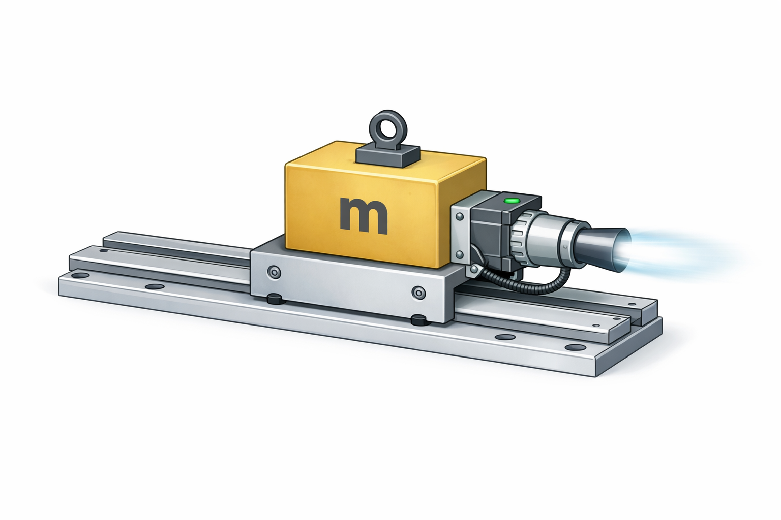
The Physical System
We apply our position control system on a block of mass, attached to a rail with a little rocket engine controlled by PID. Here is how it may look like in your imagination:
The corresponding system of ODE follows:
system = {
  x''[t] == u[t]/m,
  x'[0] == 0,
  x[0] == 0
};
Sanity Check: Constant Force
Before connecting the PID controller, let's verify our system works correctly with a constant force:
DSolve[system /. {u[t_] :> 1}, x, t] {{x->Function[{t},(*FB[*)(((*SpB[*)Power[t(*|*),(*|*)2](*]SpB*))(*,*)/(*,*)(2 m))(*]FB*)]}} As expected, we get the classic parabolic motion — Newton's second law in action:
Function[{t},(*FB[*)(((*SpB[*)Power[t(*|*),(*|*)2](*]SpB*))(*,*)/(*,*)(2 m))(*]FB*)] /.{m->1.0};
Plot[%[t], {t,0,10}, AxesLabel->{"t", "x"}, Epilog->{
  Inset[Graphics3D[Rotate[{Cuboid[1.2{-1,-1,-1},1.2{1,1,0.1}], Orange, Cuboid[{-1,-1,-1},{1,1,1}]}, 30Degree, {1,0,0}], ImageSize->100, ViewPoint->{8.5,-4.5,3}], {5,15}]
}]
(*VB[*)(FrontEndRef["a165c240-03c0-4d6a-8f80-a227fd593da0"])(*,*)(*"1:eJxTTMoPSmNkYGAoZgESHvk5KRCeEJBwK8rPK3HNS3GtSE0uLUlMykkNVgEKJxqamSYbmRjoGhgnG+iapJgl6lqkWRjoJhoZmaelmFoapyQaAAB7QBVg"*)(*]VB*) Connecting the P Controller
Now let's connect our control signal to the position through the error function. The error is the difference between the target position and the current position:
Here is our ODE:
system = {
  u[t]==(*SbB[*)Subscript[K(*|*),(*|*)"p"](*]SbB*) e[t],
  x''[t] == u[t]/m + 1,
  x'[0] == 0,
  x[0] == 0,

  e[t] == (a - x[t])
};
Solve it analytically:
sol = DSolve[system, {u,x,e}, t] // Flatten;
sol = Simplify[sol, Assumptions->{Element[a, Reals], m > 0, (*SbB[*)Subscript[K(*|*),(*|*)"p"](*]SbB*) > 0}];
x /. sol/. {m -> 1.0, a -> 1.0} /. {{(*SbB[*)Subscript[K(*|*),(*|*)"p"](*]SbB*) -> 1}, {(*SbB[*)Subscript[K(*|*),(*|*)"p"](*]SbB*) -> 0.01}};
Plot[
#[t]&/@%//Evaluate, {t,0,10},
Epilog->{Dashed, Red, Line[{{0,1.0}, {10,1.0}}]},
PlotLegends->Placed[{"Regulated", "Unregulated"}, {0.15,0.5}]
] (*VB[*)(Legended[ToExpression[FrontEndRef["4fd0fce2-abda-45e3-b237-f68534ce252e"], InputForm], Placed[LineLegend[{Directive[Opacity[1.], RGBColor[0.24, 0.6, 0.8], AbsoluteThickness[2]], Directive[Opacity[1.], RGBColor[0.95, 0.627, 0.1425], AbsoluteThickness[2]]}, {"Regulated", "Unregulated"}, LegendMarkers -> None, LabelStyle -> {}, LegendLayout -> "Column"], {0.15, 0.5}, Identity]])(*,*)(*"1:eJylUU0vA0EYXt9aJPgBEonrJrLb4iIbtESyVbrlPrvzTk26ZprZWfQH+BFc3fyCnrk7uLhKuIhE+AdmZ1qyLg7ew5N5v5953sWQN8iIZVnJjIIjCmcViLhAkotgQkV8aAHDDhnOSooKqpiqXFZIhrLYvIJtwZmsMlw9hyiVKIwhWFLhEsHLJALHRiFGdqkMrh067qpNVtbKbkklyg6YwaMKGqlqm8wegHCdxV0dbYoUDL9xBfsxigCTsQEZnzIwDH/m+DSRpqOgoEIFRJKegmGbfaneQRGVXWFp+/BMsd68s7nFYy5Eb+Hi7aB37wlX27Mnri4ze/XMmDkFG2HC41RC85hGbQZJQjMK/91MtL174ubzoRbOvnhivfh43Vm//XtzToGgoJVspTGSgIMp5R0yMfDzquvTGxlrSLRBJDq1x9mv8xjNUQhxILsxECuneb50+numj7o8lUF2P/XH9ITlmfY1vvP6sjx5WpFdDEwqsb4AQk+tFw=="*)(*]VB*) Notice the oscillations! With only proportional control, the system overshoots and oscillates around the target. This is exactly where the D and I terms become essential.
Extending to PID
Here we can no longer have an analytical solution, therefore we use NDSolve:
system = {
  (u')[t]==e[t] ((*SbB[*)Subscript[K(*|*),(*|*)"i"](*]SbB*))+((*SbB[*)Subscript[K(*|*),(*|*)"p"](*]SbB*)) (e')[t]+((*SbB[*)Subscript[K(*|*),(*|*)"d"](*]SbB*)) (e'')[t],
  u[0] == ((*SbB[*)Subscript[K(*|*),(*|*)"p"](*]SbB*)) (a - x[0]),
  x''[t] == u[t]/m + 1.0,
  x'[0] == 0.,
  x[0] == 0.,

  e[t] == (a - x[t])
};

ClearAll[sol];
sol[p_, i_, d_] := Flatten@NDSolve[system /. {m -> 5.0, a -> 2.5, (*SbB[*)Subscript[K(*|*),(*|*)"p"](*]SbB*) -> p, (*SbB[*)Subscript[K(*|*),(*|*)"i"](*]SbB*) -> i p, (*SbB[*)Subscript[K(*|*),(*|*)"d"](*]SbB*) -> d p}, {u,x,e}, {t,0,200}];
Let's make it interactive
Manipulate[
 With[{eqs = {Clip[x[t],{-0.5,4}]+0.05, Clip[0.01 u[t],{-0.5,4}]} /. sol[10.0,i,d]},
   Plot[eqs, {t,0,50},  Frame->True, PlotLegends->{"x[t]", "u[t]"}, FrameLabel->{"t (time)", "value"}, Epilog->{Dashed, Red, Line[{{0,2.5}, {50,2.5}}]},
   PlotRange->{{-1,50}, {-1,4.5}}]
 ]
,
  {{i, 0, "I"}, 0, 0.1, 0.025},
  {{d, 0, "D"}, 0, 1.0, 0.25},
  ContinuousAction->True,
  Appearance->None
]
(*VB[*)(FrontEndRef["53935cc0-d312-4ed3-b821-80321e483580"])(*,*)(*"1:eJxTTMoPSmNkYGAoZgESHvk5KRCeEJBwK8rPK3HNS3GtSE0uLUlMykkNVgEKmxpbGpsmJxvophgbGumapKYY6yZZGBnqWhgYGxmmmlgYm1oYAAB3JhSo"*)(*]VB*) As you can see:
D damps the oscillations (over-regulation), while I eliminates the systematic error.
Even more interactive version
To achieve that, we need to do the integration iteratively (again!):
Discretize it:
{
  u[t] == (*SbB[*)Subscript[K(*|*),(*|*)"p"](*]SbB*) e[t] + (*SbB[*)Subscript[K(*|*),(*|*)"i"](*]SbB*) (*TB[*)Integrate[(*|*)e[\[Tau]](*|*), {(*|*)\[Tau](*|*),(*|*)0(*|*),(*|*)t(*|*)}](*|*)(*1:eJxTTMoPSmNmYGAo5gUSYZmp5S6pyflFiSX5RcGcQBHPvJLUdCA3NZMRpIgFSIQUlaYCAIJ9Dew=*)(*]TB*) + (*SbB[*)Subscript[K(*|*),(*|*)"d"](*]SbB*) e'[t],
  x''[t] == u[t]/m,
  x'[0] == 0,
  x[0] == 0,

  e[t] == (a - x[t])
}
Lift the integral:
{
  u'[t] == (*SbB[*)Subscript[K(*|*),(*|*)"p"](*]SbB*) e'[t] + (*SbB[*)Subscript[K(*|*),(*|*)"i"](*]SbB*) e[t] + (*SbB[*)Subscript[K(*|*),(*|*)"d"](*]SbB*) e''[t],
  x''[t] == u[t]/m,
  x'[0] == 0,
  x[0] == 0,

  e[t] == (a - x[t])
}
Remove 2nd order:
{
  h[t] == e'[t],
  u'[t] == (*SbB[*)Subscript[K(*|*),(*|*)"p"](*]SbB*) h[t] + (*SbB[*)Subscript[K(*|*),(*|*)"i"](*]SbB*) e[t] + (*SbB[*)Subscript[K(*|*),(*|*)"d"](*]SbB*) h'[t]
}
Discretize:
{
  h[t] == e'[t],
  u'[t] == (*SbB[*)Subscript[K(*|*),(*|*)"p"](*]SbB*) h[t] + (*SbB[*)Subscript[K(*|*),(*|*)"i"](*]SbB*) e[t] + (*SbB[*)Subscript[K(*|*),(*|*)"d"](*]SbB*) h'[t]
} /. {(e_)'[t] :> (*FB[*)((e[n]-e[n-1])(*,*)/(*,*)(\[Delta]t))(*]FB*), e_[t] :> e[n]};
(dsol = Solve[%, {h[n],u[n]}]//Flatten)//FullSimplify//TableForm
(*GB[*){{h[n]->(*FB[*)((-e[-1+n]+e[n])(*,*)/(*,*)(\[Delta]t))(*]FB*)}(*||*),(*||*){u[n]->(*FB[*)((-e[-1+n] ((*SbB[*)Subscript[K(*|*),(*|*)"d"](*]SbB*)+\[Delta]t ((*SbB[*)Subscript[K(*|*),(*|*)"p"](*]SbB*)))+e[n] ((*SbB[*)Subscript[K(*|*),(*|*)"d"](*]SbB*)+\[Delta]t (\[Delta]t ((*SbB[*)Subscript[K(*|*),(*|*)"i"](*]SbB*))+(*SbB[*)Subscript[K(*|*),(*|*)"p"](*]SbB*)))+\[Delta]t (-h[-1+n] ((*SbB[*)Subscript[K(*|*),(*|*)"d"](*]SbB*))+u[-1+n]))(*,*)/(*,*)(\[Delta]t))(*]FB*)}}(*]GB*) Define a constructor for our discrete PID controller and automatically apply our solution:
createPID := Module[{uState, hState, eState}, With[{
  rules1 = dsol,
  rules2 = {
    e[n-1] -> Indexed[eState, 2],
    e[n] -> Indexed[eState, 1],

    h[n-1] -> Indexed[hState, 2],
    h[n] -> Indexed[hState, 1],

    u[n-1] -> Indexed[uState, 2],
    u[n] -> Indexed[uState, 1],

    \[Delta]t -> #5,
    (*SbB[*)Subscript[K(*|*),(*|*)"d"](*]SbB*) -> #4,
    (*SbB[*)Subscript[K(*|*),(*|*)"p"](*]SbB*) -> #2,
    (*SbB[*)Subscript[K(*|*),(*|*)"i"](*]SbB*) -> #3
  }
},
  Hold@Module[{},

    uState = {0,0};
    hState = {0,0};
    eState = {0,0};

    (
      eState[[2]] = eState[[1]];
      eState[[1]] = #1;

      hState[[2]] = hState[[1]];
      hState[[1]] = h[n];

      uState[[2]] = uState[[1]];
      uState[[1]] = u[n]
    )&
  ] /. rules1 /. rules2
] ] // ReleaseHold;
Now we have a constructor, let's create!
pid = createPID; One could potentially reduce each integration step to a simple matrix multiplication, since the coefficients remain constant.
Now we can solve it iteratively:
pid[0.1, 0.1,0.1,0.1,0.1] -0.08900000000000002%60 Now we have our discretized controller, let's make a test subject:
{
  x''[t] == u[t]/m,
  x'[0] == 0,
  x[0] == 0,

  e[t] == (a - x[t])
}
Following the same procedure:
{
  v'[t] == u[t]/m,
  x'[t] == v[t],
  e[t] == (a - x[t])
} /. {
  v'[t] -> (*FB[*)((v[n] - v[n-1])(*,*)/(*,*)(\[Delta]t))(*]FB*),
  v[t] -> v[n],
  x'[t] -> (*FB[*)((x[n] - x[n-1])(*,*)/(*,*)(\[Delta]t))(*]FB*),
  x[t] -> x[n],
  e[t] -> e[n]
}//Simplify;

Solve[%, {v[n], x[n], e[n]}]//Flatten//TableForm
(*GB[*){{v[n]->-(*FB[*)((-\[Delta]t u[t]-m v[-1+n])(*,*)/(*,*)(m))(*]FB*)}(*||*),(*||*){x[n]->-(*FB[*)((-((*SpB[*)Power[\[Delta]t(*|*),(*|*)2](*]SpB*)) u[t]-m \[Delta]t v[-1+n]-m x[-1+n])(*,*)/(*,*)(m))(*]FB*)}(*||*),(*||*){e[n]->-(*FB[*)((-a m+((*SpB[*)Power[\[Delta]t(*|*),(*|*)2](*]SpB*)) u[t]+m \[Delta]t v[-1+n]+m x[-1+n])(*,*)/(*,*)(m))(*]FB*)}}(*]GB*) Here we can do it manually since it is quite simple system of equations:
testSystem[initialPos_, mass_] := Module[{stateV = {0., 0.}, stateX = {1.,1.} initialPos},
  Function[{u, target, dt},
    stateV[[2]] = stateV[[1]];
    stateV[[1]] = If[Abs[stateX[[1]]] > 1, -stateV[[1]], stateV[[2]] + (*FB[*)((dt)(*,*)/(*,*)(mass))(*]FB*) u];
    stateX[[2]] = stateX[[1]];
    stateX[[1]] = Clip[stateX[[2]] + dt stateV[[1]], {-0.9,0.9}, {-0.88, 0.88}];

    {stateX[[1]], target - stateX[[1]]}
  ]
];
Don't forget to add boundary conditions, that our block will bounce off the wall and won't shoot into space. Let's test it under the constant force and then flip it to slow down back to the original state:
sys = testSystem[0., 1.0];
Table[sys[1, 0., 0.01][[1]], {10}];
Join[%, Table[sys[0., 0., 0.01][[1]], {100}]];
Join[%, Table[sys[-1.0, 0., 0.01][[1]], {10}]];
Join[%, Table[sys[0., 0., 0.01][[1]], {100}]];
ListLinePlot[%]
(*VB[*)(FrontEndRef["f11c2e35-61ae-4f47-a09e-0bb036019505"])(*,*)(*"1:eJxTTMoPSmNkYGAoZgESHvk5KRCeEJBwK8rPK3HNS3GtSE0uLUlMykkNVgEKpxkaJhulGpvqmhkmpuqapJmY6yYaWKbqGiQlGRibGRhamhqYAgCDkRUv"*)(*]VB*) Great! Now we are ready to assemble.
Putting it all together
Again the same scheme, but the target position is no longer stationary, but controlled by a user's input in real time:
Let's go!
pid = createPID;
sys = testSystem[0., 1.0];

Module[{
  value = 0.0,
  error = 0.0,
  target = 0.5,
  control = 0.0,
  gravity = 0.25,
  history = Table[{i,0.}, {i,300}],
  p = <|"P" -> 1.0, "I" -> 0.0, "D" -> 0.0|>,
  handler
},
  handler = Function[Null,
    {value, error} = sys[Clip[pid[error, p["P"], p["I"], p["D"], 0.1], {-10,10}] - gravity, target, 0.1];
    history[[1,2]] = error;
    history = Transpose[{history[[All,1]], RotateLeft[history[[All,2]]]}];
  ];

 Row[{EventHandler[Graphics[{
    Red, Line[{{-1,target}, {1, target}}] // Offload,
    Blue, Line[{{-1,value}, {1, value}}] // Offload,
    EventHandler[AnimationFrameListener[value // Offload], handler]
  }, PlotRange->{{-1,1}, {-1,1}}, ImageSize->{100,300}], {"mousemove" -> Function[xy,
    target = Clip[xy[[2]], {-0.8,0.8}];
  ]}],
    Graphics[Line[history // Offload], PlotRange->{{1,300}, {-1,1}}, ImageSize->{200,300}, Axes->True, AxesOrigin->{0,0.00001}, Ticks->{False, True}, "TransitionType"->None, Frame->True, PlotLabel->"Error"],
    EventHandler[InputGroup[<|
      "P" -> InputRange[0, 2.0, 0.01, p["P"], "Label"->"P"],
      "I" -> InputRange[0, 2.0, 0.01, p["I"], "Label"->"I"],
      "D" -> InputRange[0, 2.0, 0.01, p["D"], "Label"->"D"]
    |>], Function[data, p = data]]
  }]

]
Try it yourself. You will notice that D is essential to reduce oscillations and I to compensate for gravity.
Self-balancing Robot
Let's make something cool!
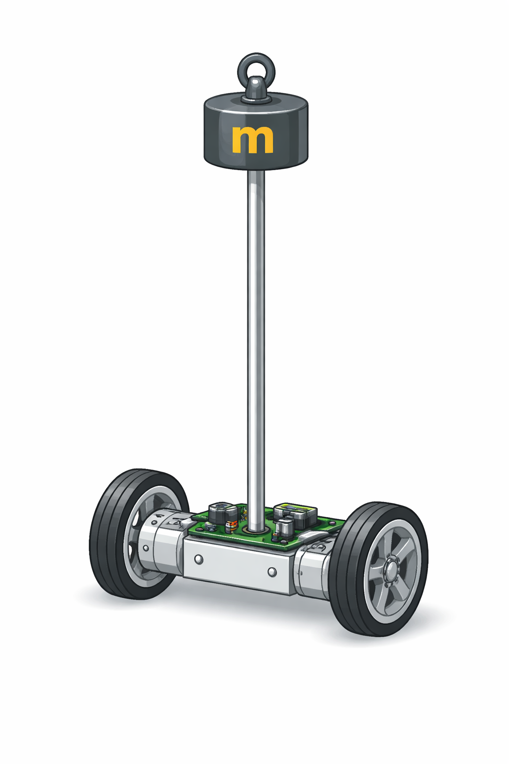
Before diving into the full robot, let's build up from simpler systems.
Newton's 2nd Law for Rotational Motion
Let's have a look at the simplest rotational system—a pendulum:
Then we solve motion equation for rotation:
restricting ourselves to one coordinate:
Now if we move our origin to the moving (accelerating) frame, i.e.
the effect will appear as some phantom moment of force in the moving frame:
To complete the picture, let's add friction as well:
Let's create a system of equations for that:
createPendulum[i\[Theta]_, g_, l_, d_:0.1] := Module[{\[Omega] = {0., 0.}, \[Theta] = {1.,1.} i\[Theta]},
  Function[{ax, dt},
    \[Omega][[2]] = \[Omega][[1]];
    \[Omega][[1]] = (1.0 - d) \[Omega][[2]] + (*FB[*)((dt g)(*,*)/(*,*)(l))(*]FB*) Sin[\[Theta][[1]]] + (*FB[*)((dt ax)(*,*)/(*,*)(l))(*]FB*) Cos[\[Theta][[1]]];
    \[Theta][[2]] = \[Theta][[1]];
    \[Theta][[1]] = \[Theta][[2]] + dt \[Omega][[1]];

    \[Theta][[1]]
  ]
];
Let's see how unstable it is:
pen = createPendulum[0.01, 9.9, 1.0, 0.003];
Module[{pos = {0,1.0}, t = 0.0}, Animate[
  t = pen[0.0, 0.1];
  pos = {Sin[t], Cos[t]};
  Graphics[{Line[{{0,0}, pos}], Disk[pos, 0.05]}, PlotRange->{{-1,1}, {-1,1}}, AxesOrigin->{0.00001,0}, Axes->True, Ticks->None]
, {dummy, 0, 0.5, 0.01}, Appearance->None]]
(*VB[*)(FrontEndRef["097f178b-de59-4ed6-a091-e938dc08bc62"])(*,*)(*"1:eJxTTMoPSmNkYGAoZgESHvk5KRCeEJBwK8rPK3HNS3GtSE0uLUlMykkNVgEKG1iapxmaWyTppqSaWuqapKaY6SYaWBrqploaW6QkG1gkJZsZAQCD+xW1"*)(*]VB*) Now what if we apply a constant acceleration to one of the sides:
pen = createPendulum[0.01, 9.9, 1.0, 0.03];
Module[{pos = {0,1.0}, t = 0.0}, Animate[
  t = pen[30.0, 0.1];
  pos = {Sin[t], Cos[t]};
  Graphics[{{Red,Arrow[{{0,0}, {0.8,0}}]}, Line[{{0,0}, pos}], Disk[pos, 0.05]}, PlotRange->{{-1,1}, {-1,1}}, AxesOrigin->{0.00001,0}, Axes->True, Ticks->None]
, {dummy, 0, 0.5, 0.01}, Appearance->None]]
(*VB[*)(FrontEndRef["26d78d07-a987-49ef-a975-873f1807789e"])(*,*)(*"1:eJxTTMoPSmNkYGAoZgESHvk5KRCeEJBwK8rPK3HNS3GtSE0uLUlMykkNVgEKG5mlmFukGJjrJlpamOuaWKamAVnmproW5sZphhYG5uYWlqkAe/sVFQ=="*)(*]VB*) Wheels for the Robot
What about our vehicle? The PID controller will certainly control the voltage of the motors or current...
In electric motors (especially DC), voltage determines speed (velocity/RPM) and current determines torque (loading force).
Then we go with voltage. The revolutions of a wheel will be directly transferred to the coordinate:
createPlatform[initialPos_, mass_] := Module[{stateV = {0., 0.}, stateX = {1.,1.} initialPos},
  Function[{u, dt},
    stateV[[2]] = stateV[[1]];
    (* stateV[[1]] = If[Sign[stateV[[2]]] Sign[u] > 0, Sign[u] Max[Abs[u], Abs[stateV[[2]]]], u]; *)
    stateV[[1]] = If[Abs[Abs[stateX[[1]]] - 2.0] < 0.01, 0, u];
    stateX[[2]] = stateX[[1]];
    stateX[[1]] = Clip[stateX[[2]] + dt stateV[[1]], {-2,2}];

    {stateX[[1]], (*FB[*)((stateV[[1]] - stateV[[2]])(*,*)/(*,*)(dt))(*]FB*)}
  ]
];
We made it in a way that if the platform goes too far, the motors will stop spinning (vehicle got trapped):
Module[{
  platform = createPlatform[0.0, 3.0],
  pen = createPendulum[0.00, 9.9, 1.0, 0.003],
  x = .0,
  ac = .0,
  voltage = .0,
  pos = {0., 0.},
  angle = 0.0,
  handler
},

  handler = Function[Null,
    {x, ac} = platform[voltage, 0.01];
    angle = pen[-ac, 0.01];
    pos = {Sin[angle], Cos[angle]};
  ];

  EventHandler[Graphics[{
    Translate[{{Brown, Disk[{0,-0.8+1.0}, 0.1]},
      Rectangle[{-0.4,-1.0+0.2+1.0}, {0.4,-1.0+0.4+1.0}],
      Red, Line[{{0,0.4}, pos// Offload}], Disk[pos// Offload, 0.05]
    }, {x,-0.1 - 1.0} // Offload],
    Line[{{-2.0, -1.0}, {2, -1.0}}],
    EventHandler[AnimationFrameListener[x//Offload], handler]
  }, PlotRange->{{-2,2}, {-1,1}}, ImageSize->{400,200}], {
    "mousemove" -> Function[xy, voltage = 2.0 xy[[1]]]
  }]
]
You can't keep it stable with just your mouse!
Add PID Controller
Let's add a PID controller for the angular position, so it will drive our motors to keep the angle of the pendulum at 0. This can be illustrated as:
However, in order to control the position of our robot, we can add a bias voltage to the motors:
Here is our assembled code:
Module[{p = <|"P" -> 11.71, "I" -> 36.56, "D" -> 0|>}, Module[{
  platform = createPlatform[0.0, 1.0],
  pid = createPID,
  pid2 = createPID,
  pen = createPendulum[0.01, 9., 1.0, 0.03],
  x = .0,
  ac = .0,

  target = 0.0,
  voltage = .0,
  pos = {0., 0.},
  angle = 0.0,
  history = Table[{i,0.}, {i,300}],
  handler
},

  handler = Function[Null,

    voltage = Clip[pid[angle, p["P"], p["I"], p["D"], 2 0.02], {-15,15}];
    voltage = Clip[pid[angle, p["P"], p["I"], p["D"], 2 0.02], {-15,15}];
    {x, ac} = platform[ voltage + 2.0 (x-target), 2 0.02];
    angle = pen[-ac, 2 0.02];
    {x, ac} = platform[ voltage + 2.0 (x-target), 2 0.02];
    angle = pen[-ac, 2 0.02];
    pos = {Sin[angle], Cos[angle]};
    history[[1,2]] = voltage;
    history = Transpose[{history[[All,1]], RotateLeft[history[[All,2]]]}];
  ];

  Row[{EventHandler[Graphics[{
    Translate[{{Brown, Disk[{0,-0.8+1.0}, 0.1]},
      Rectangle[{-0.4,-1.0+0.2+1.0}, {0.4,-1.0+0.4+1.0}],
      Red, Line[{{0,0.4}, pos// Offload}], Disk[pos// Offload, 0.05]
    }, {x,-0.1 - 1.0} // Offload],
    Line[{{-2.0, -1.0}, {2, -1.0}}],
    EventHandler[AnimationFrameListener[pos//Offload], handler],
    Green, Arrow[{{target, -1.2}, {target, -1.0}} // Offload]
  },
    "TransitionType"->None,
    PlotRange->{{-2,2}, {-1- 0.2,1- 0.2}}, ImageSize->{400,200}], {
    "mousemove" -> Function[xy,
      target = 0.6 target + 0.4 xy[[1]]
    ]
  }],

  Graphics[Line[history // Offload], PlotRange->{{1,300}, {-2,2}}, ImageSize->{200,300}, Axes->True, AxesOrigin->{0,0.00001}, Ticks->{False, True}, "TransitionType"->None, Frame->True, PlotLabel->"Voltage"],
    Column[{Button["Reset",
      platform = createPlatform[0.0, 1.0];
      pid = createPID;
      pen = createPendulum[0.01, 9., 1.0, 0.03];
      ac = .0;
      voltage = .0;
      angle = 0.0;

    ], EventHandler[InputGroup[<|
      "P" -> InputRange[0, 40.0, 0.01, p["P"], "Label"->"P"],
      "I" -> InputRange[0, 40.0, 0.01, p["I"], "Label"->"I"],
      "D" -> InputRange[0, 10.0, 0.01, p["D"], "Label"->"D"]
    |>], Function[data, p = data]]}]
  }]
] ]
As you can see, I and P are the most critical here. Our system is highly non-linear: pendulum rotation is coupled to linear motion through the motor. This makes it quite different from the heater or the block-on-a-rail we examined earlier.
It would be great to test one in real life.
Behind every basic device — heaters, motors, e-scooters — lie beautiful and clever ideas carefully crafted by engineers and scientists. What a time to be alive.
Embrace the power of knowledge!
Cheers, Kirill