Fireflies or Nature's Cellular Automaton
Have you ever wondered how each firefly knows when to blink? How do they coordinate across the fields and trees? I guess we're heading towards a many-body problem here.
This blog post was originally inspired by a beautiful piece written by physicist Cian Luke Martin: "Fireflies, Magnets and Emergence". He demonstrates a very clear way of modeling the collective behavior of fireflies at night—as a sort of cellular automaton. I couldn't help but think: I should try this out!
Have you ever wondered how each firefly knows when to blink? How do they coordinate across the fields and trees?
Well, I guess we're heading towards a many-body problem...
Following Cian's basic model, each firefly needs:
- an internal state or clock
- a flash (and a sensor)
The last component indicates the end of the internal clock cycle and broadcasts to all other fireflies so they can synchronize their clocks as well. Therefore, we can represent each firefly as a flow chart:
flowchart LR
    decayAction[Decay]
    decayCheck{Decayed?}
    flash[Flash]
    adjust[Adjust]

    decayAction --> decayCheck
    decayCheck -- Yes --> flash
    decayCheck -- No --> adjust
    adjust --> decayAction
    flash --> adjust
TLDR; If you really want to see the final result:
Module[{f = RandomReal[{0,1.01}, {25,25}]}, Refresh[

  f = Map[Clip[# - 0.01, {0.0,1.0}, {1.0,1.0}]&, f, {2}];

  f = Clip[f + (2.0 Round[f] - 1.0) Clip[ListConvolve[{{1.0,1.0,1.0},{1.0,0.0,1.0},{1.0,1.0,1.0}}, Floor[f], 2, 0], {0,  0.001}], {0., 1.0}];

  ArrayPlot[f, Frame->True, ColorFunction->"PlumColors"]
, 1/30.0]]
The question is: how does it adjust itself? There are multiple models for this case. We'll pick the simplest approach, assuming that:
- the cycle duration of each firefly is the same and fixed;
- when a flash emitted by another firefly is seen, the internal phase or clock is adjusted forward or backward slightly, depending on which is closer.
In this model, our fireflies are out of phase initially and are trying to align with each other. Since the visibility of another firefly's flash signal depends on distance, we can naturally limit the number of "visible" neighbors—limiting the interaction distance.
Let's define a function that will distribute n points over a given region:
generateFireFlies[n_:200, region_:Rectangle[{-10,-10}, {10,10}]] := fireFlies = With[{
  pos = RandomPoint[region, n]
},
  Transpose[{pos, Table[ RandomReal[{0,1.0}], {Length[pos]}]}]
];
Here, a firefly is represented as a list of two objects:
position;state- a real-valued number (randomly generated):
generateFireFlies[1] // First %7B%7B-5.896003641067651%60%2C1.7548145516864455%60%7D%2C0.1972596724287563%60%7D For the next step, we find all nearest fireflies and bake all the connections within a given radius into a connectionMatrix:
bakeConnections[r_:3.7] := (
  connectionMatrix = Table[
  If[i==j, Infinity, (*SpB[*)Power[Norm[i[[1]] - j[[1]]](*|*),(*|*)2](*]SpB*)]
, {i, fireFlies}, {j, fireFlies}];
  connectionMatrix = MapIndexed[Function[{value, index},
  If[value < r, index[[1]], Nothing]
], #] &/@ connectionMatrix
);
For example, if we generate 10 fireflies and highlight all neighbors:
generateFireFlies[10, Disk[{0,0},10]];
bakeConnections[30.0];
Graphics[{
  Blue, Table[
    Line[{fireFlies[[i,1]], fireFlies[[#,1]]}]&/@connectionMatrix[[i]],
    {i,Length[fireFlies]}
  ],
  Red, Disk@@#&/@fireFlies
}, ImageSize->250]
(*VB[*)(FrontEndRef["41d66f5c-464c-42d3-90cd-a22ed5e23d6e"])(*,*)(*"1:eJxTTMoPSmNkYGAoZgESHvk5KRCeEJBwK8rPK3HNS3GtSE0uLUlMykkNVgEKmximmJmlmSbrmpiZAAmjFGNdS4PkFN1EI6PUFNNUI+MUs1QAgegV0A=="*)(*]VB*) Do you remember our flow chart? Flashing and decaying are rather simple: we count down our state from 1.0 to 0.0, and once 0 is reached, we reset it back to 1.0—our flash signal. Here we define all 3 functions we need:
decay[{pos_, state_}] := {pos, Clip[state - 0.01, {0,1}]};
flash[{pos_, state_}] := {pos, If[state == 0, 1, state]};
adjust[{pos_, 0}, index_] := {pos, 0}
adjust[{pos_, state_}, index_] := With[{i = index[[1]]},
 {pos, If[Or@@Thread[fireFlies[[connectionMatrix[[i]], 2]] == 1],
   Clip[state + Sign[2 Round[state] - 1] 0.0001, {0,1}],
   state
 ]}
]
adjust is the most interesting one, since we also need to scan over all visible neighbors and then, if one is in the "flashing" state (1.0), we push our internal clock forward or backward depending on which is closer to the flashing state of 1.0.
Now we create a global cycle:
update = Function[Null,
  fireFlies = decay /@ fireFlies;
  fireFlies = flash /@ fireFlies;
  fireFlies = MapIndexed[adjust, fireFlies];
];
2 Fireflies
We'll take our time and start small, using only 2 units. This will make it much easier for us to actually see how the synchronization happens.
generateFireFlies[2, Circle[{0,0},0.5]];
bakeConnections[2.0];
fireFlies %7B%7B%7B-0.29375610430108234%60%2C-0.40460765092352324%60%7D%2C0.7153475734585732%60%7D%2C%7B%7B-0.4866072033546407%60%2C0.11494968309384473%60%7D%2C0.5494089476223747%60%7D%7D Let's also track their states as an XY graph and see how it evolves. The radius of the dots will represent the state: largest radius means flash.
generateFireFlies[2, Circle[{0,0},0.5]];
bakeConnections[2.0];

radii = fireFlies[[All,2]];
history = {Table[{i, 0}, {i,200}], Table[{i, 0}, {i,200}]};

{Graphics[{
  Circle[fireFlies[[1]][[1]], radii[[1]]//Offload],
  Circle[fireFlies[[2]][[1]], radii[[2]]//Offload],
  EventHandler[AnimationFrameListener[radii//Offload], Function[Null,
    update[];
    update[];
    radii = 0.5 fireFlies[[All,2]];

    history[[1,1,2]] = fireFlies[[1,2]];
    history[[2,1,2]] = fireFlies[[2,2]];
    history = {
      Transpose[{history[[1,All,1]], RotateLeft[history[[1,All,2]], 1]}],
      Transpose[{history[[2,All,1]], RotateLeft[history[[2,All,2]], 1]}]
    };
  ]]
}, TransitionType->None, "Controls"->False,
ImageSize->250,
PlotRange->{{-1,1}, {-1,1}}], Graphics[{
  ColorData[97][1], Line[history[[1]] // Offload],
  ColorData[97][2], Line[history[[2]] // Offload]
}, Axes->True, Frame->True, "Controls"->False,
  PlotRange->{{0,200}, {0,1}},
  TransitionType->None,
  ImageSize->250
]}//Row
(*GB[*){{(*VB[*)(Graphics[{Circle[{0.19356814455530394, -0.4610112508534005}, Offload[radii[[1]]]], Circle[{-0.4834763306808521, -0.1274779889682111}, Offload[radii[[2]]]], AnimationFrameListener[Offload[radii], "Event" -> "341d536c-7305-4add-9f35-37dc23e29b79"]}, TransitionType -> None, "Controls" -> False, ImageSize -> 250, PlotRange -> {{-1, 1}, {-1, 1}}])(*,*)(*"1:eJxTTMoPSmNkYGAoZgESHvk5KWmsIB4HkHAvSizIyEwuTmOGyftkFpekMYF4bEDCObMoOSc1FaQbJNZ5ysTz+rET9pfNE0JNG+/uhxjLDiT809Jy8hNTIDpB5gQkFpUUg+wpSkzJzMwEKcRp7MQWra1uH+/tt2M79cAo8AAJxjLBjRUDEo55mbmJJZn5eW5FibmpIJ+k5qUWYZiG0I8wN6g0JzUYJO5alppXEqwCZBmbGKaYGpsl65obG5jqmiSmpOhaphmb6hqbpyQbGacaWSaZW6IaUMwHZIQUJeYVZ4JcEVJZkAqW88vPS0WzChT4zvl5JUX5OcVg97gl5hSjKSrmBDI8cxPTU4Mzq1Izf8H9iqIgICe/JCgxLx1JMyIOYbzM/0CAFAmY4gD7VIWl"*)(*]VB*)(*|*),(*|*)(*VB[*)(Graphics[{RGBColor[0.368417, 0.506779, 0.709798], Line[Offload[history[[1]]]], RGBColor[0.880722, 0.611041, 0.142051], Line[Offload[history[[2]]]]}, Axes -> True, Frame -> True, "Controls" -> False, PlotRange -> {{0, 200}, {0, 1}}, TransitionType -> None, ImageSize -> 250])(*,*)(*"1:eJxTTMoPSmNkYGAoZgESHvk5KWnsIB4HkHAvSizIyEwuTmOByftkFpekMcPkg9ydnPNz8ouKCqZNeqoy5bp9keG0l9M7zB/YFx1vmeG9atsze4TRPpl5qRAeyHz/tLSc/MSUNCaYdEBiUQlYJgNoRX5RZSZIKRarfI5EP7+v98a+6F/1h1tLex/bF22etU59l94hCqwCySCkg0pzUsEMx4rUYjAjpKg0FU2eFchwK0rMTcWhIBjkaOf8vJKi/JxiiOrEnGJ0UzhBrsnJLwlKzEtHkgOHMgovE0gzZJ5AcSdCnBHT/XxgVyXmFWeWZObnhVQWQBzql5+HzQ2euYnpqcGZVamZv4A8AGemgaE="*)(*]VB*)}}(*]GB*) It takes a few cycles to make them fully in sync.
Going Bigger
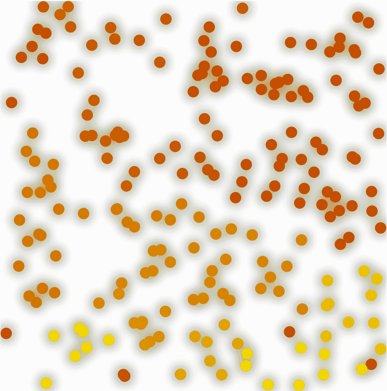
What about 200 of them? For this, we should change our visualization to pure colors flashing and blend between two:
Table[Blend[{Darker[Red], Yellow}, i], {i,0,1,0.25}] {(*VB[*)(RGBColor[0.6666666666666666, 0., 0.])(*,*)(*"1:eJxTTMoPSmNiYGAo5gUSYZmp5S6pyflFiSX5RcEsQBHn4PCQNGaQPAeQCHJ3cs7PyS8qCgWDp/ZFDFAAZwAAECkROQ=="*)(*]VB*),(*VB[*)(RGBColor[0.75, 0.25, 0.])(*,*)(*"1:eJxTTMoPSmNiYGAo5gUSYZmp5S6pyflFiSX5RcEsQBHn4PCQNGaQPAeQCHJ3cs7PyS8qYgCDF/ZQxgUYg4EBAOzrEE0="*)(*]VB*),(*VB[*)(RGBColor[0.8333333333333333, 0.5, 0.])(*,*)(*"1:eJxTTMoPSmNiYGAo5gUSYZmp5S6pyflFiSX5RcEsQBHn4PCQNGaQPAeQCHJ3cs7PyS8qWgUGr+yLGMDgAYzBwAAAS3QUWw=="*)(*]VB*),(*VB[*)(RGBColor[0.9166666666666666, 0.75, 0.])(*,*)(*"1:eJxTTMoPSmNiYGAo5gUSYZmp5S6pyflFiSX5RcEsQBHn4PCQNGaQPAeQCHJ3cs7PyS8qCgWDt/ZFDGDwAsZgYAAAHTcSaA=="*)(*]VB*),(*VB[*)(RGBColor[1., 1., 0.])(*,*)(*"1:eJxTTMoPSmNiYGAo5gUSYZmp5S6pyflFiSX5RcEsQBHn4PCQNGaQPAeQCHJ3cs7PyS8qYgCDD/boDAYGAO7rEHU="*)(*]VB*)} Visualize it:
generateFireFlies[200, Rectangle[{-10,-10}, {10,10}]];
bakeConnections[3.7];

cf = (List@@Blend[{Darker[Red], Yellow}, #])&;
colors = cf /@ fireFlies[[All,2]];

Graphics[{
  Table[With[{i=i, xy = fireFlies[[i,1]]},{
    RGBColor[colors[[i]]],
    Disk[xy, 0.3]
  } // Offload], {i, Length[fireFlies]}],
  EventHandler[AnimationFrameListener[colors // Offload],
    Function[Null,
      update[];
      colors = cf /@ fireFlies[[All,2]];
    ]
  ]
}, Background->Black]
For authenticity, we can duplicate the layer of our fireflies and blur it—this will create a nice halo-like effect.
With[{fires = Table[With[{i=i, xy = fireFlies[[i,1]]},{
    RGBColor[colors[[i]]],
    Disk[xy, 0.3]
  } // Offload], {i, Length[fireFlies]}]},
    {
      SVGAttribute[SVGGroup[fires], "style"->"filter: blur(10px)"],
      fires
    }
  ]
What beautiful patterns they form! It's time to prepare some nice hot tea, turn off the lights, and enjoy the spectacle from nature.
Cellular Automaton
If we go to a bigger scale and evenly distribute our small bugs on a grid, we eventually get something similar to this:
ArrayPlot[#, ImageSize -> 40, Mesh -> True] & /@
 CellularAutomaton["GameOfLife", {(*GB[*){{0(*|*),(*|*)1(*|*),(*|*)0}(*||*),(*||*){0(*|*),(*|*)0(*|*),(*|*)1}(*||*),(*||*){1(*|*),(*|*)1(*|*),(*|*)1}}(*||*)(*1:eJxTTMoPSmNkYGAo5gUSYZmp5S6pyflFiSX5RcFsQBHfxJKizAoAs04KOA==*)(*]GB*), 0}, 8]
{(*VB[*)(FrontEndRef["a137289f-663f-4ce6-b182-92e1511769f2"])(*,*)(*"1:eJxTTMoPSmNkYGAoZgESHvk5KRCeEJBwK8rPK3HNS3GtSE0uLUlMykkNVgEKJxoamxtZWKbpmpkZp+maJKea6SYZWhjpWhqlGpoaGpqbWaYZAQB6JhTy"*)(*]VB*),(*VB[*)(FrontEndRef["650010c5-2241-45d8-bb30-499584b6e227"])(*,*)(*"1:eJxTTMoPSmNkYGAoZgESHvk5KRCeEJBwK8rPK3HNS3GtSE0uLUlMykkNVgEKm5kaGBgaJJvqGhmZGOqamKZY6CYlGRvomlhamlqYJJmlGhmZAwBq8RR7"*)(*]VB*),(*VB[*)(FrontEndRef["171400de-c5ed-442c-92fd-4e8d01ec19ea"])(*,*)(*"1:eJxTTMoPSmNkYGAoZgESHvk5KRCeEJBwK8rPK3HNS3GtSE0uLUlMykkNVgEKG5obmhgYpKTqJpumpuiamBgl61oapQFZqRYpBoapyYaWqYkAguUV+g=="*)(*]VB*),(*VB[*)(FrontEndRef["e8a87950-4ca6-41cc-a511-9e6a3c6d8923"])(*,*)(*"1:eJxTTMoPSmNkYGAoZgESHvk5KRCeEJBwK8rPK3HNS3GtSE0uLUlMykkNVgEKp1okWphbmhromiQnmumaGCYn6yaaGhrqWqaaJRonm6VYWBoZAwCDMRV6"*)(*]VB*),(*VB[*)(FrontEndRef["29bd0311-c3f6-44c4-87af-095f8d997b68"])(*,*)(*"1:eJxTTMoPSmNkYGAoZgESHvk5KRCeEJBwK8rPK3HNS3GtSE0uLUlMykkNVgEKG1kmpRgYGxrqJhunmemamCSb6FqYJ6bpGliaplmkWFqaJ5lZAAB+MxVZ"*)(*]VB*),(*VB[*)(FrontEndRef["ab804e76-d61e-44f3-b0db-0cf42bd34cbf"])(*,*)(*"1:eJxTTMoPSmNkYGAoZgESHvk5KRCeEJBwK8rPK3HNS3GtSE0uLUlMykkNVgEKJyZZGJikmpvpppgZpuqamKQZ6yYZpCTpGiSnmRglpRibJCelAQCLKhZU"*)(*]VB*),(*VB[*)(FrontEndRef["4e38000c-ba28-4bbe-afc0-709c342107b8"])(*,*)(*"1:eJxTTMoPSmNkYGAoZgESHvk5KRCeEJBwK8rPK3HNS3GtSE0uLUlMykkNVgEKm6QaWxgYGCTrJiUaWeiaJCWl6iamJRvomhtYJhubGBkamCdZAACFiBWM"*)(*]VB*),(*VB[*)(FrontEndRef["e6c10e18-1932-4b77-8d42-771c48f8c0a7"])(*,*)(*"1:eJxTTMoPSmNkYGAoZgESHvk5KRCeEJBwK8rPK3HNS3GtSE0uLUlMykkNVgEKp5olGxqkGlroGloaG+maJJmb61qkmBjpmpsbJptYpFkkGySaAwB5XBUc"*)(*]VB*),(*VB[*)(FrontEndRef["2bbf69e2-9119-4147-8a3e-f22f79d6282f"])(*,*)(*"1:eJxTTMoPSmNkYGAoZgESHvk5KRCeEJBwK8rPK3HNS3GtSE0uLUlMykkNVgEKGyUlpZlZphrpWhoaWuqaGJqY61okGqfqphkZpZlbppgZWRilAQB/1RVW"*)(*]VB*)} A cellular automaton consists of a regular grid of cells, each in one of a finite number of states, such as on and off (in contrast to a coupled map lattice). The grid can be in any finite number of dimensions. For each cell, a set of cells called its neighborhood is defined relative to the specified cell.
However, in our case, instead of plain on and off states, we have a range [1..0], and the automaton rules are not discrete either. One can formulate such a rule as:
If one or more of the nearest neighbors is "infinitely" close to the "flashing" state (i.e., to 1.0), then we add or subtract a small number from the state of the current cell.
We need to break this down into a set of simple and parallel operations over arrays. Doing it in a procedural style, as we did before, would be quite inefficient and would kill performance.
Think Like a Shader
Okay, neighbor scanning sounds like a list convolution with a 2D kernel. However, to detect only "flashing" cells, we can round them to the lowest integer beforehand:
field%20%3D%20RandomReal%5B%7B0%2C1.01%7D%2C%20%7B25%2C25%7D%5D%3B%0A%0AArrayPlot%5B%0A%20%20field%20%2B%20Floor%5Bfield%5D%2C%20%0A%20%20ColorFunction-%3EFunction%5B%28%2ATB%5B%2A%29Piecewise%5B%7B%7B%28%2A%7C%2A%29%28%2AVB%5B%2A%29%28RGBColor%5B1%2C%201%2C%200%5D%29%28%2A%2C%2A%29%28%2A%221%3AeJxTTMoPSmNiYGAo5gUSYZmp5S6pyflFiSX5RcEsQBHn4PCQNGaQPAeQCHJ3cs7PyS8qYgCDD%2FboDAYGAO7rEHU%3D%22%2A%29%28%2A%5DVB%2A%29%28%2A%7C%2A%29%2C%28%2A%7C%2A%29%231%3E0.7%60%28%2A%7C%2A%29%7D%2C%7B%28%2A%7C%2A%29GrayLevel%5B%231%5D%28%2A%7C%2A%29%2C%28%2A%7C%2A%29True%28%2A%7C%2A%29%7D%7D%5D%28%2A%7C%2A%29%28%2A1%3AeJxTTMoPSmNiYGAo5gUSYZmp5S6pyflFiSX5RcGcQJGAzNTk1PLM4tRMkCIAD2QL0A%3D%3D%2A%29%28%2A%5DTB%2A%29%5D%2C%0A%20%20PlotLabel-%3E%22Cells%20in%20a%20flashing%20state%22%2C%0A%20%20Frame-%3ETrue%0A%5D%0A%0Ac%20%3D%20Clip%5BListConvolve%5B%28%2AGB%5B%2A%29%7B%7B1.0%28%2A%7C%2A%29%2C%28%2A%7C%2A%291.0%28%2A%7C%2A%29%2C%28%2A%7C%2A%291.0%7D%28%2A%7C%7C%2A%29%2C%28%2A%7C%7C%2A%29%7B1.0%28%2A%7C%2A%29%2C%28%2A%7C%2A%290.0%28%2A%7C%2A%29%2C%28%2A%7C%2A%291.0%7D%28%2A%7C%7C%2A%29%2C%28%2A%7C%7C%2A%29%7B1.0%28%2A%7C%2A%29%2C%28%2A%7C%2A%291.0%28%2A%7C%2A%29%2C%28%2A%7C%2A%291.0%7D%7D%28%2A%7C%7C%2A%29%28%2A1%3AeJxTTMoPSmNkYGAo5gUSYZmp5S6pyflFiSX5RcFsQBHfxJKizAoAs04KOA%3D%3D%2A%29%28%2A%5DGB%2A%29%2C%20Floor%5Bfield%5D%2C%202%2C%200%5D%2C%20%7B0%2C0.01%7D%5D%3B%0A%28%2ABB%5B%2A%29%28%2A%20plot%20it%20%2A%29%28%2A%2C%2A%29%28%2A%221%3AeJxTTMoPSmNhYGAo5gcSAUX5ZZkpqSn%2BBSWZ%2BXnFaYwgCS4g4Zyfm5uaV%2BKUXxEMUqxsbm6exgSSBPGCSnNSg9mAjOCSosy8dLBYSFFpKpoKkDkeqYkpEFXBILO1sCgJSczMQVYCAOFrJEU%3D%22%2A%29%28%2A%5DBB%2A%29%0AArrayPlot%5B%0A%20%20field%20%2B%20300%20c%2C%20%0A%20%20ColorFunction-%3EFunction%5B%28%2ATB%5B%2A%29Piecewise%5B%7B%7B%28%2A%7C%2A%29%28%2AVB%5B%2A%29%28RGBColor%5B1%2C%200%2C%200%5D%29%28%2A%2C%2A%29%28%2A%221%3AeJxTTMoPSmNiYGAo5gUSYZmp5S6pyflFiSX5RcEsQBHn4PCQNGaQPAeQCHJ3cs7PyS8qYgCDD%2FZQBgMDnAEA4iUPRg%3D%3D%22%2A%29%28%2A%5DVB%2A%29%28%2A%7C%2A%29%2C%28%2A%7C%2A%29%231%3E0.7%60%28%2A%7C%2A%29%7D%2C%7B%28%2A%7C%2A%29GrayLevel%5B%231%5D%28%2A%7C%2A%29%2C%28%2A%7C%2A%29True%28%2A%7C%2A%29%7D%7D%5D%28%2A%7C%2A%29%28%2A1%3AeJxTTMoPSmNiYGAo5gUSYZmp5S6pyflFiSX5RcGcQJGAzNTk1PLM4tRMkCIAD2QL0A%3D%3D%2A%29%28%2A%5DTB%2A%29%5D%2C%0A%20%20PlotLabel-%3E%22Cells%20affected%20by%20flashes%22%2C%0A%20%20Frame-%3ETrue%0A%5D (*VB[*)(FrontEndRef["a14f0d1e-ae02-424b-9c50-29232777a69b"])(*,*)(*"1:eJxTTMoPSmNkYGAoZgESHvk5KRCeEJBwK8rPK3HNS3GtSE0uLUlMykkNVgEKJxqapBmkGKbqJqYaGOmaGJkk6VommxroGlkaGRuZm5snmlkmAQCCxxU3"*)(*]VB*) (*VB[*)(FrontEndRef["7676e411-3f7a-4e34-baa2-459af299fd83"])(*,*)(*"1:eJxTTMoPSmNkYGAoZgESHvk5KRCeEJBwK8rPK3HNS3GtSE0uLUlMykkNVgEKm5uZm6WaGBrqGqeZJ+qapBqb6CYlJhrpmphaJqYZWVqmpVgYAwB80RWB"*)(*]VB*) These red cells are affected by the central one in the "flashing" state. We clip the result as well to make it independent of the number of flashing cells.
On the next step, we need to determine whether to add or subtract time from their state. We can find a nice solution by combining Clip and Round operations on arrays:
%0Ac%20%3D%20Clip%5BListConvolve%5B%28%2AGB%5B%2A%29%7B%7B1.0%28%2A%7C%2A%29%2C%28%2A%7C%2A%291.0%28%2A%7C%2A%29%2C%28%2A%7C%2A%291.0%7D%28%2A%7C%7C%2A%29%2C%28%2A%7C%7C%2A%29%7B1.0%28%2A%7C%2A%29%2C%28%2A%7C%2A%290.0%28%2A%7C%2A%29%2C%28%2A%7C%2A%291.0%7D%28%2A%7C%7C%2A%29%2C%28%2A%7C%7C%2A%29%7B1.0%28%2A%7C%2A%29%2C%28%2A%7C%2A%291.0%28%2A%7C%2A%29%2C%28%2A%7C%2A%291.0%7D%7D%28%2A%7C%7C%2A%29%28%2A1%3AeJxTTMoPSmNkYGAo5gUSYZmp5S6pyflFiSX5RcFsQBHfxJKizAoAs04KOA%3D%3D%2A%29%28%2A%5DGB%2A%29%2C%20Floor%5Bfield%5D%2C%202%2C%200%5D%2C%20%7B0%2C%20%200.001%7D%5D%3B%0Ac%20%3D%20%282.0%20Round%5Bfield%5D%20-%201.0%29%20%2A%20c%3B%0A%0A%28%2ABB%5B%2A%29%28%2A%20plot%20it%20%2A%29%28%2A%2C%2A%29%28%2A%221%3AeJxTTMoPSmNhYGAo5gcSAUX5ZZkpqSn%2BBSWZ%2BXnFaYwgCS4g4Zyfm5uaV%2BKUXxEMUqxsbm6exgSSBPGCSnNSg9mAjOCSosy8dLBYSFFpKpoKkDkeqYkpEFXBILO1sCgJSczMQVYCAOFrJEU%3D%22%2A%29%28%2A%5DBB%2A%29%0A%0AArrayPlot%5B%0A%20%20field%20%2B%203000%20c%2C%20%0A%20%20ColorFunction-%3EFunction%5B%28%2ATB%5B%2A%29Piecewise%5B%7B%7B%28%2A%7C%2A%29%28%2AVB%5B%2A%29%28RGBColor%5B1%2C%200%2C%200%5D%29%28%2A%2C%2A%29%28%2A%221%3AeJxTTMoPSmNiYGAo5gUSYZmp5S6pyflFiSX5RcEsQBHn4PCQNGaQPAeQCHJ3cs7PyS8qYgCDD%2FZQBgMDnAEA4iUPRg%3D%3D%22%2A%29%28%2A%5DVB%2A%29%28%2A%7C%2A%29%2C%28%2A%7C%2A%29%231%3E0.7%60%28%2A%7C%2A%29%7D%2C%7B%28%2A%7C%2A%29%28%2AVB%5B%2A%29%28RGBColor%5B0%2C%200%2C%201%5D%29%28%2A%2C%2A%29%28%2A%221%3AeJxTTMoPSmNiYGAo5gUSYZmp5S6pyflFiSX5RcEsQBHn4PCQNGaQPAeQCHJ3cs7PyS8qYoACdMYHewDM1w9G%22%2A%29%28%2A%5DVB%2A%29%28%2A%7C%2A%29%2C%28%2A%7C%2A%29%231%3C0.3%60%28%2A%7C%2A%29%7D%2C%7B%28%2A%7C%2A%29GrayLevel%5B%231%5D%28%2A%7C%2A%29%2C%28%2A%7C%2A%29True%28%2A%7C%2A%29%7D%7D%5D%28%2A%7C%2A%29%28%2A1%3AeJxTTMoPSmNiYGAo5gUSYZmp5S6pyflFiSX5RcGcQJGAzNTk1PLM4tRMZiAPAA9oC9E%3D%2A%29%28%2A%5DTB%2A%29%5D%2C%0A%20%20PlotLabel-%3E%22Cells%20affected%20by%20flashes%20%28forward%20and%20backward%29%22%2C%0A%20%20Frame-%3ETrue%0A%5D (*VB[*)(FrontEndRef["87efb1eb-93e1-4367-8c6c-7bfa99545181"])(*,*)(*"1:eJxTTMoPSmNkYGAoZgESHvk5KRCeEJBwK8rPK3HNS3GtSE0uLUlMykkNVgEKW5inpiUZpibpWhqnGuqaGJuZ61okmyXrmielJVpampqYGloYAgCKphWL"*)(*]VB*) Great! Now we know how to efficiently update all affected cells. The decay and flash functions are rather trivial to implement using a Clip and Subtract composition mapped over all elements:
Module[{f = field}, Refresh[
  (*BB[*)(* here we go *)(*,*)(*"1:eJxTTMoPSmNhYGAo5gcSAUX5ZZkpqSn+BSWZ+XnFaYwgCS4g4Zyfm5uaV+KUXxEMUqxsbm6exgSSBPGCSnNSg9mAjOCSosy8dLBYSFFpKpoKkDkeqYkpEFXBILO1sCgJSczMQVYCAOFrJEU="*)(*]BB*)
  f = Map[Clip[# - 0.01, {0.0,1.0}, {1.0,1.0}]&, f, {2}];

  ArrayPlot[f, Frame->True, ColorFunction->"AvocadoColors"]
, 1/30.0]]
Final Version
Now let's combine everything together!
Module[{f = RandomReal[{0,1.01}, {25,25}]}, Refresh[
  (*BB[*)(* here we go *)(*,*)(*"1:eJxTTMoPSmNhYGAo5gcSAUX5ZZkpqSn+BSWZ+XnFaYwgCS4g4Zyfm5uaV+KUXxEMUqxsbm6exgSSBPGCSnNSg9mAjOCSosy8dLBYSFFpKpoKkDkeqYkpEFXBILO1sCgJSczMQVYCAOFrJEU="*)(*]BB*)
  f = Map[Clip[# - 0.01, {0.0,1.0}, {1.0,1.0}]&, f, {2}];

  f = Clip[f + (2.0 Round[f] - 1.0) Clip[ListConvolve[(*GB[*){{1.0(*|*),(*|*)1.0(*|*),(*|*)1.0}(*||*),(*||*){1.0(*|*),(*|*)0.0(*|*),(*|*)1.0}(*||*),(*||*){1.0(*|*),(*|*)1.0(*|*),(*|*)1.0}}(*||*)(*1:eJxTTMoPSmNkYGAo5gUSYZmp5S6pyflFiSX5RcFsQBHfxJKizAoAs04KOA==*)(*]GB*), Floor[f], 2, 0], {0,  0.001}], {0., 1.0}];

  ArrayPlot[f, Frame->True, ColorFunction->"PlumColors"]
, 1/30.0]]
After ~4 minutes of waiting we get this:
Since we picked a rectangular convolution kernel for detecting neighbor flashes, the stabilizing patterns and flashing waves look somewhat rectangular. In reality, however, bugs are not arranged in a grid and may also have different cycles as well as more complex behaviors related to mating, etc. I believe this is a nice virtual experiment for researching collective behavior beyond discrete cellular automata.
Optimized Version
Using Refresh together with ArrayPlot is good for prototyping, but carries a lot of overhead for each update cycle. To get the best results in terms of performance you need to write it in C, we need Image. Instead of relying on a plotting function, we directly feed the GPU texture with our field array using NumericArray as a proxy. This will also allow us to increase the field size.
field = RandomReal[{0,1.0}, {50,50}];

render = Function[Null,
  Do[

  field = Map[Clip[#- 0.01, {0.0,1.0}, {1.0,1.0}]&, field, {2}];
  field = Clip[field + (2.0 Round[field] - 1.0) Clip[ListConvolve[(*GB[*){{1.0(*|*),(*|*)1.0(*|*),(*|*)1.0}(*||*),(*||*){1.0(*|*),(*|*)0.0(*|*),(*|*)1.0}(*||*),(*||*){1.0(*|*),(*|*)1.0(*|*),(*|*)1.0}}(*||*)(*1:eJxTTMoPSmNkYGAo5gUSYZmp5S6pyflFiSX5RcFsQBHfxJKizAoAs04KOA==*)(*]GB*), Floor[field], 2, 0], {0,  0.001}], {0., 1.0}]; , {2}];


  imageBuffer = NumericArray[255.0 field, "Byte", "ClipAndRound"];
];

render[];

Image[imageBuffer // Offload, "Byte", Epilog->EventHandler[
  AnimationFrameListener[imageBuffer // Offload],
  render
], Magnification->20, Antialiasing->False]
After lots of iterations, we eventually get a "radar," literally... Try this initial state I saved for you:
field = NotebookRead[NotebookStore["haphazard-0e9"]]; Render to a Video
Since we're already working with image data, it's super easy to make a movie out of it:
val = 1.0;
PrintTemporary[ProgressIndicator[val//Offload, {1, 60 10}]]
movie = Table[
  val++;
  render[];
  ImageResize[Colorize[Image[imageBuffer]], Scaled[6], Method->"NearestNeighbor"],
  {60 10}
];
And now we export it as a video:
FrameListVideo[movie, FrameRate->60]