Animation

Basic

Way 1

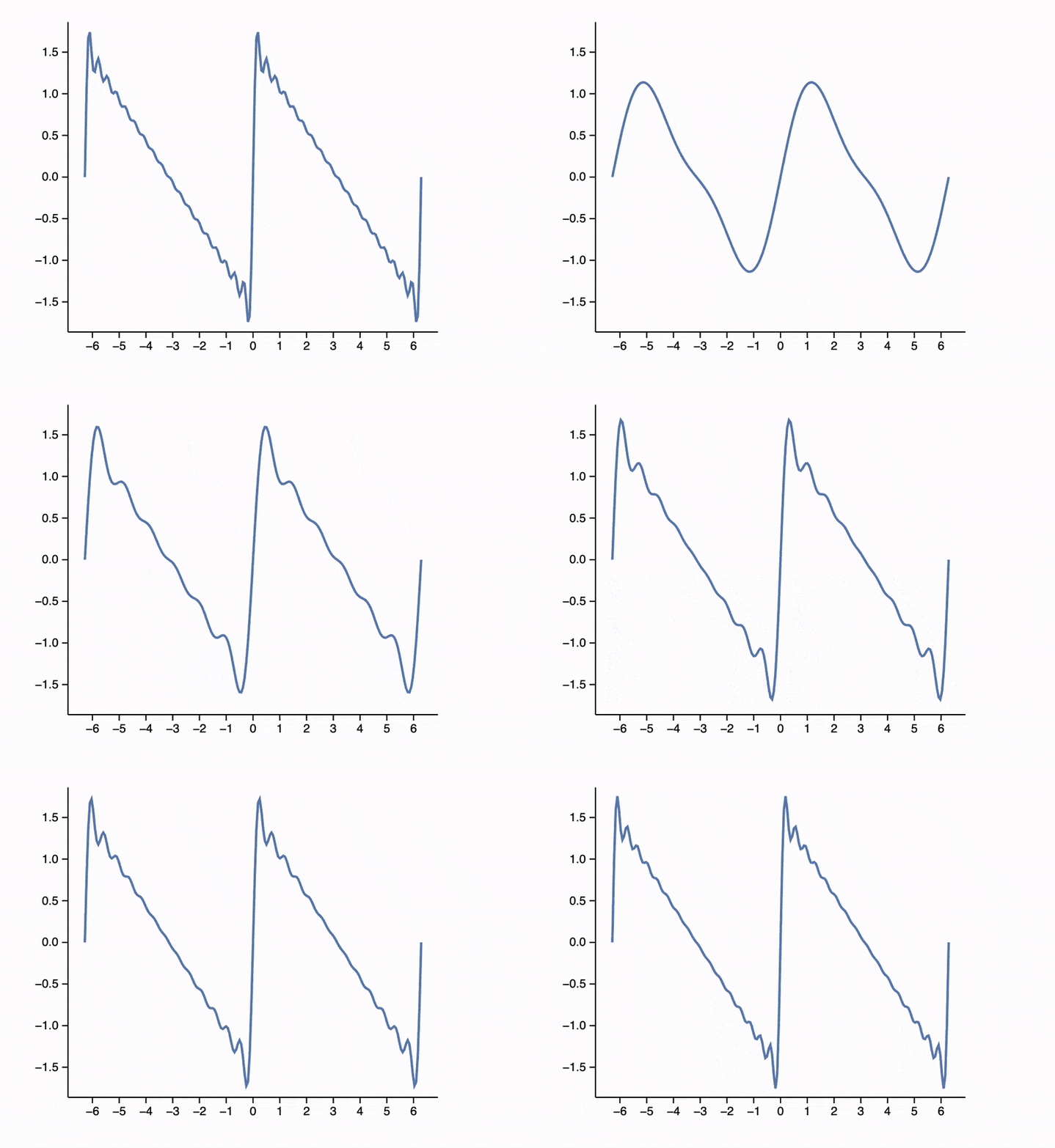
Use AnimatePlot for plot-like animations

AnimatePlot[Sum[Sin[x w]/w, {w, 1,n}] // Re, {x, -2Pi,2Pi}, {n, 1,20, 1}]

Way 2

Use Animate for animating arbitrary expressions

Animate[Row[{Sin[x], "==", Series[Sin[x], {x,0,n}], Invisible[1/2]}], {n, 1, 10, 1}, AnimationRate->3]

here we used Invisible with a dummy expression to keep the height of the editor the same. The result will look like

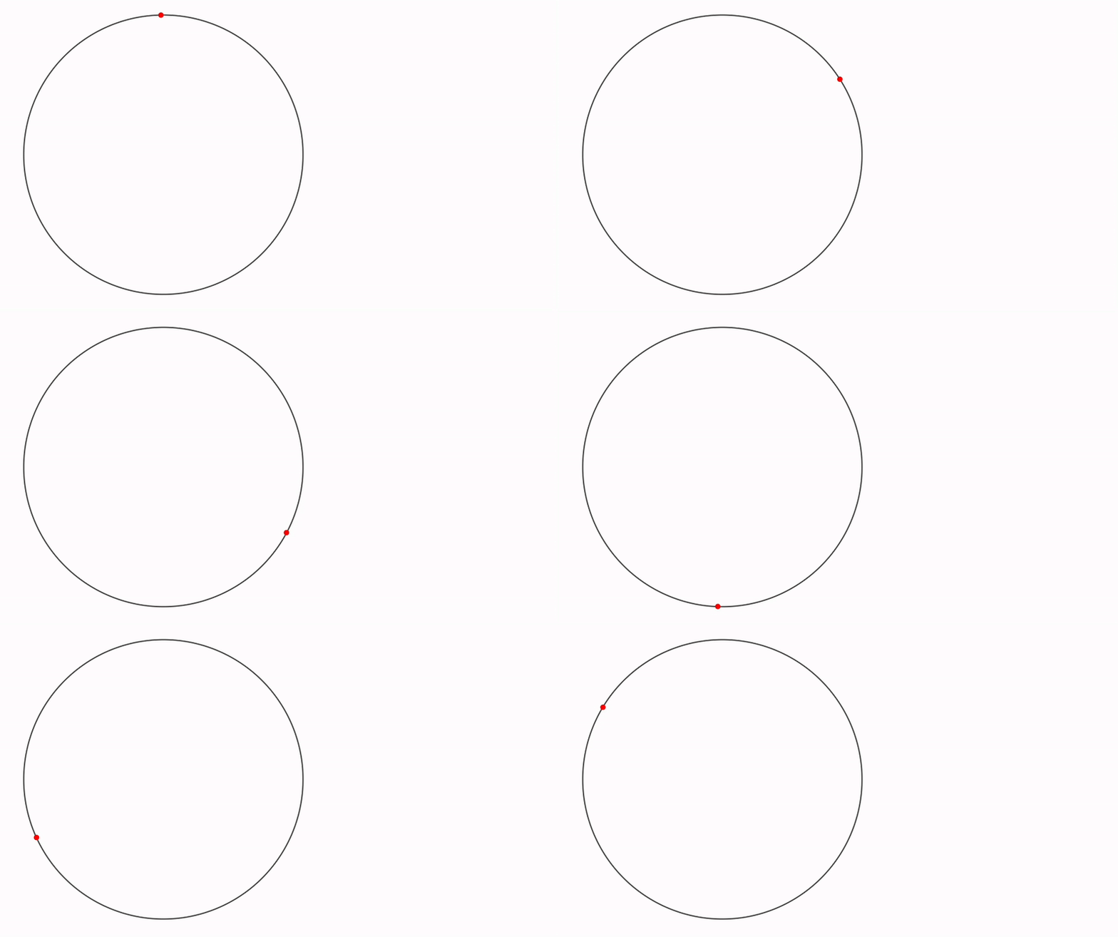
Using UpdateFunction option, one can bypass the default update method and write your own using [[Offload]]

Module[{pts},
  Animate[Graphics[{
    Circle[{0,0},1],
    Red, Point[pts // Offload]
  }, ImageSize->Small], {t, 0, 2Pi, 0.1}, 
  "UpdateFunction" -> Function[t,
    pts = {Sin[t], Cos[t]};
    False
  ]]
]

Smoother version

There are two way how to make the previous example look smoother.

1. Native Graphics's data interpolation

Module[{pts},
  Animate[Graphics[{
    Circle[{0,0},1],
    Red, Point[pts // Offload]
  }, ImageSize->Small,
    TransitionDuration->220
  ], {t, 0, 2Pi, 0.1}, 
  "UpdateFunction" -> Function[t,
    pts = {Sin[t], Cos[t]};
    False
  ]]
]

2. Increate the update frame rate

Module[{pts},
  Animate[Graphics[{
    Circle[{0,0},1],
    Red, Point[pts // Offload]
  }, ImageSize->Small,
    TransitionType->None
  ], {t, 0, 2Pi, 0.02}, 
  "UpdateFunction" -> Function[t,
    pts = {Sin[t], Cos[t]};
    False
  ], AnimationRate->60]
]

It is important to disable interpolation, since it will only hurt the performance at higher rates.

Advanced

Way 1

Consider using to achieve the highest frame rate and smooth animations.

• AnimationFrameListener for Graphics
• AnimationFrameListener for Graphics3D

Use TransitionType set to None if the calculation time does not exceed 1/60 seconds. Otherwise, consider using the "Linear" interpolation option and a small value for TransitionDuration, around 10-100, depending on how long it takes to update the data.

tip

If your animation looks choppy, you can use JavaScript to interpolate between data changes over time. Use TransitionType and TransitionDuration.

For example:

cell 1

balls = RandomReal[{-1,1}, {100,3}];
vels  = RandomReal[{-1,1}, {100,3}];

Graphics3D[{
  Table[With[{i = i},
    {
      RGBColor[RandomReal[{0,1}, 3]],
      Sphere[balls[[i]] // Offload, 0.03]
    }
  ], {i, Length[balls]}], 
  AnimationFrameListener[balls // Offload, "Event"->"frame"]
}]

Evaluate the cell above. It will create a canvas with randomly scattered balls.

At the start of the browser's frame, an event "frame" is triggered to request an update of data from the Kernel. However, after this, you'll need to "recharge" AnimationFrameListener, or else it will not trigger the event again. This can be automated to occur whenever a change in the balls symbol is detected.

This process ensures the following benefits:

• Synchronization of animation with the browser's engine (eliminating flickering).
• The ability to skip frames if recalculations take longer than one frame of your browser, adapting to your computing power.

Here is our update function:

EventHandler["frame", Function[Null,

  vels = Table[
    If[Norm[balls[[i]]] < 0.01, -1, 1] vels[[i]] - 0.08 balls[[i]]
  , {i, Length[balls]}];
  
  balls = Table[balls[[i]] + 0.08 vels[[i]], {i, Length[balls]}];
]];

To start the animation, reevaluate cell 1 or use this "kickstarter":

EventFire["frame", Null]

Way 2

Consider using SetInterval for resource-intensive animations. Set TransitionDuration and TransitionType to appropriate values for interpolation.

Usually, if your SetInterval is, let's say, 100 ms, then TransitionDuration should also be around 100 ms to achieve the smoothest animation.

tip

If your animation looks choppy, you can use JavaScript to interpolate between data portions over time. Use TransitionType and TransitionDuration.

For example:

ParametricAnimator[equation_, variable_:t, range_:{0, Infinity, 0.1}] := LeakyModule[{time = range[[1]], task, scale = 1, array = {}, scaledArray={}, cell = ResultCell[]},

    (* Sample the equation each frame and rescale if needed *)
    animate := Block[{variable = time},
        With[{e = {Sin[t], Cos[t]} equation},
            scale = If[Norm[e scale] > 1.4, scale 0.95, scale 1];
            array = Append[array, e];
            scaledArray = scale array; 
            pointer = e scale;
        ];

        time += range[[3]];
        If[time >= range[[2]], TaskRemove[task]];
    ];

    animate;

    (* Async task to animate every 50 ms *)
    task = SetInterval[animate, 50];

    (* Stop the task if the cell is destroyed or reevaluated *)
    EventHandler[cell, {"Destroy"->Function[Null, TaskRemove[task]; Print["removed"]]}];

    Graphics[{Red, PointSize[0.05], Point[pointer // Offload],
 Opacity[0.5], Line[scaledArray // Offload]
  }, TransitionDuration->50, TransitionType->"Linear", "Controls"->False, PlotRange->{{-1,1}, {-1,1}}]
]

This will sample a given parametric equation and animate it with a 50 ms time step, while on JavaScript's side, it will interpolate between frames so that the overall animation appears smooth and is rendered at 60FPS.

ParametricAnimator[Exp[Sin[t]] - 2 Cos[4t] + Sin[(2t - Pi)/24], t, {0,16, 0.05}]

Way 3

If your animation depends on user interaction, it might be best to update object attributes only when an event occurs.

For example:

pt = {0,0};
Graphics[{
    White,
    EventHandler[
        Rectangle[{-2,-2}, {2,2}],
        {"mousemove"->Function[xy, pt = xy]}
    ],
    PointSize[0.05], Cyan,
    Point[pt // Offload]
}]

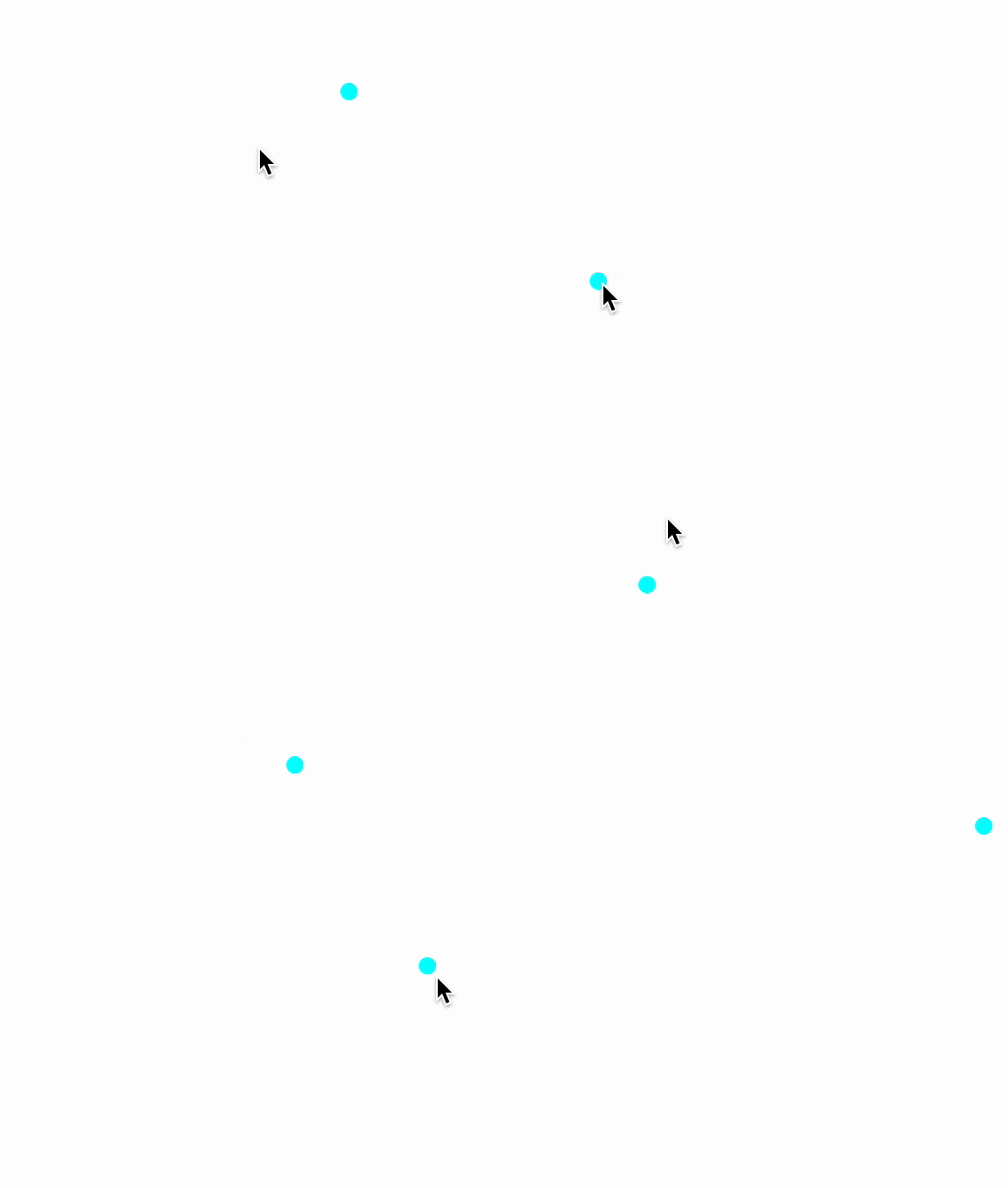
A mouse follower.

A remark on color and opacity

RGBColor and Opacity support updates in the context of Graphics. However, all graphics symbols sharing the same scope should bind to them indirectly. The good news is that you do not have to worry about this—just use them normally.

color = {1,0,0};
Graphics[{RGBColor[color // Offload], Disk[{0,0}, 1]}]

EventHandler[InputJoystick[], Function[xy,
    color = Normalize[{xy[[1]], xy[[2]], 0.5}] // Abs;
]]

Animating Bubbles

We can go further and animate bubbles. The problem arises when we create a bubble. In fact, we need to provide a graphical primitive (let’s say Disk) and a dynamic symbol to control its properties (see Dynamics). Creating 1000 dynamic symbols is a significant overhead for the system, especially if we want to update all of them.

Pool of Objects

Let us use a limited number of dynamic symbols—buffers—and bind each animated Disk or bubble to one of its parts.

cPool = Table[{0., 0.}, {i, 100}]; (* Positions *)
vPool = cPool; (* Velocities *)
rPool = Table[0., {i, 100}]; (* Radius or lifetime *)

oPool = Table[Null, {i, 100}]; (* References to objects *)

The general idea is not to allocate new variables for each new object but rather to reuse objects from the pool.

The graphical output remains the same:

scene = FrontInstanceReference[];
Graphics[{White, EventHandler[Rectangle[{-1, -1}, {1, 1}], {"mousemove" -> handler[scene]}], scene}, ImagePadding -> None]

Our future animation loop will look like this:

handler[scene_] := Function[xy, 
  If[!created[xy, scene], update[]];
];

We don't need to evaluate it now.

The update function iterates over our arrays and produces new values:

update[] := With[{},
  {cPool, rPool} = Transpose[MapIndexed[Function[{a, index},
    (* If the slot is not empty, recalculate *)
    If[oPool[[index // First]] =!= Null,
      
      If[a[[2]] <= 0.002, 
        (* If the radius is too small, remove the object *)
        remove[index // First];
        a
      ,
        (* Otherwise, animate *)
        {a[[1]] + 0.05 vPool[[index // First]], 0.9 a[[2]]}
      ]
    ,
      a
    ]
  ], {cPool, rPool} // Transpose]];
];

If the lifetime is close to zero, we need to remove the created instance and free up slots in our buffers for new objects:

remove[index_] := (
  (* Destroy the instance on the frontend *)
  Delete[oPool[[index]]]; 
  oPool[[index]] = Null
);

And finally, a function to create new objects:

created[xy_, scene_] := With[{
  (* Find an empty slot *)
  slot = FirstPosition[oPool, Null]
},
  If[!MissingQ[slot],
    With[{s = slot // First},

      (* Initialize positions, radius, etc. *)
      cPool[[s]] = xy;
      rPool[[s]] = 0.05;
      vPool[[s]] = RandomReal[{-1, 1}, 2];
      oPool[[s]] = True;

      (* Update so the object doesn't appear abruptly *)
      update[];

      (* Create an instance of Disk in the graphics *)
      With[{
        group = FrontInstanceGroup[],
        o = {
          Hue[RandomReal[{0, 1}], 1, 1],
          (* Prevent double updates *)
          Disk[Offload[cPool[[s]]], Offload[rPool[[s]], "Static" -> True]]
        }
      },
        oPool[[s]] = group;
        FrontSubmit[o // group, scene];
      ];
    ];

    True
  ,
    False
  ]
]

The key difference from the previous example Simple Example is that we track our created instances using FrontInstanceGroup, allowing us to remove them later from our SVG canvas (also known as Graphics).

All positions and radii are stored in two solid symbols, cPool and rPool. This means we only need to perform two data transactions with our frontend, significantly saving resources when animating objects on the screen. The payload size matters less than the number of transactions in terms of transport load.